Read from the beginning or jump to a stable example ID. Each example includes its complete input and captured result. Copy link preserves the address of the guide you are reading, including its current domain and path.

The sixteen compositions in the pinned ROOT Asymptote atlas supply the starting ideas. This tour develops them into independent, explained programs and adds data graphics, language features, native 3D surfaces and page composition.

Every program is complete. The concise view shows the drawing operations; expand the standalone source to see its explicit imports, palette, TeX engine, white canvas and export settings. All data are synthetic and inline. Run a downloaded program with asy -noView -f pdf ASY-01-001.asy.

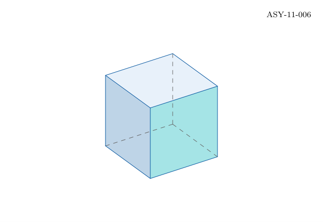
Trigonometric functions use radians. The dir constructor uses degrees. Native 3D examples use settings.render=0 and fixed cameras for printable vector projections. They have no interactive model embedded in the PDF. Explicitly projected wireframes retain all their lines; selected hidden cube edges are styled manually. Sampling a curve, integrating an ODE, choosing a projection and changing a pen are different operations.

Create your first plot

Asymptote has a command-line workflow, much like gnuplot: write a text file, run the plotting program and open the output. Its source files use .asy. You can use any text editor. The asy command compiles the drawing; a separate viewer displays the result. The optional xasy graphical editor is explained in CLI, interactive prompt and GUI.

1. Check the tools

Install Asymptote and a TeX distribution such as TeX Live or MacTeX, then check that both commands are on your terminal's PATH:

asy --version
pdflatex --version

This first example uses pdfLaTeX to typeset the axis labels. The graph module ships with Asymptote. See the official installation instructions for your platform.

2. Save a complete program

Create a working directory, open a new text file and save the following as first-plot.asy:

import graph;

size(320, 200);

real f(real x) {
    return sin(x);
}

draw(graph(f, 0, 2*pi), blue + linewidth(1));
xaxis("$x$", BottomTop, Ticks);
yaxis("$\\sin(x)$", LeftRight, Ticks);

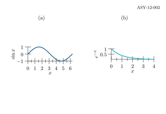
import graph loads plotting and axis helpers. f defines a real-valued function; sin uses radians. graph samples that function from zero to 2*pi, and draw draws the sampled path with the chosen pen. The axis commands add labels and ticks. size fits the figure into the requested width and height in PostScript points; one point is 1/72 inch.

3. Compile from the terminal

Change to the directory containing first-plot.asy and run:

asy -noView -tex pdflatex -f pdf first-plot.asy

The result is first-plot.pdf in the same directory. -f pdf selects the output format, -tex pdflatex selects the TeX engine, and -noView keeps the command suitable for terminal jobs and automated builds. Asymptote writes the picture at the end of this program; this minimal example needs no explicit shipout command.

4. Preview, edit and rebuild

Open the PDF in your usual viewer. To ask Asymptote to launch its configured viewer after compiling, use the capital -V option:

asy -V -tex pdflatex -f pdf first-plot.asy

Change sin(x) to cos(x), save the source and run the command again. The PDF is regenerated from the edited program. A viewer window opened by -V is a preview of the output; the drawing instructions remain in the source file. See drawing in batch mode and the graph module reference.

5. Reuse the figure

PDF is a vector output suitable for inclusion in a document. For SVG or a PNG preview, these optional Poppler commands convert the verified PDF:

pdftocairo -svg first-plot.pdf first-plot.svg
pdftocairo -png -singlefile -r 150 first-plot.pdf first-plot

The second command creates first-plot.png at 150 dpi. These converters require Poppler; they are separate from the asy compiler.

CLI, interactive prompt and GUI

Choose the interface that fits the task:

Interface	How to start	Typical use
Script / batch mode	`asy -noView -f pdf file.asy`	Rebuild figures from saved source; use shell scripts or Make.
Compile and preview	`asy -V -f pdf file.asy`	Recompile a saved program and open the result in a viewer.
Interactive prompt	`asy`	Try statements one at a time and build up a picture interactively.
Graphical editor	`xasy`, when installed	Move and edit graphical objects, then save Asymptote source.

For the minimal plot above, keep -tex pdflatex in the compilation command. The downloaded tour programs already select their TeX engine in the source.

Try the interactive prompt

Start asy without a filename. Enter these lines one at a time at its prompt:

draw((0,0)--(100,100));
erase
quit

draw adds a line and updates the displayed picture. erase clears the current picture; quit returns to the shell. These last two are special interactive commands. The prompt supports command history and completion. The interactive-mode manual describes further commands.

Use a GUI when useful

xasy is an optional graphical editor for Asymptote. It can move objects, add drawing elements and save the result as Asymptote source. Availability and dependencies depend on the installation; having asy on PATH does not guarantee that xasy is installed. See the GUI overview and GUI installation instructions. The script workflow above works independently of this editor.

How this compares with gnuplot

Task	gnuplot	Asymptote
Saved source	Plotting commands, often in a `.gp` file	A typed graphics program in a `.asy` file
Run a file	`gnuplot plot.gp`	`asy -noView -tex pdflatex -f pdf plot.asy`
Draw a function	`plot sin(x)`	`import graph;` followed by `draw(graph(sin, 0, 2*pi));`
Choose output	Terminal and output settings in the script	`-f pdf` on the CLI or settings in the source
Explore interactively	Start `gnuplot` for its prompt	Start `asy` for its prompt; use `-V` to preview saved programs

When following a worked example in this tour, download its complete Asymptote source file. The concise drawing panel omits setup such as imports, palette definitions, canvas sizing and output settings. For example:

asy -noView -f pdf ASY-01-001.asy

If asy or pdflatex is not found, check the installation and PATH. If compilation succeeds but no window appears, open the generated PDF or use -V. If a copied snippet reports undefined names, start with the complete standalone source instead of the focused drawing panel.

References and provenance

The atlas supplies the initial composition ideas. These programs use independent coordinates, fixtures and teaching explanations, and the plotting chapters add new examples. No poster builder is required. ATLAS_PANEL properties and sources/atlas-provenance.json retain the sixteen-panel mapping and pinned hash. Asymptote, TeX, Poppler and their installed libraries remain external dependencies.

01 · Paths and coordinates

ASY-01-001

Join two points

A path is a value that can be drawn with a chosen pen. Coordinate pairs describe positions in a Cartesian plane.

Back to figure overview

Asymptote drawing

draw((40,45)--(280,175),Blue+linewidth(2));
dot((40,45),Orange+4); dot((280,175),Orange+4);
label("$A$",(40,45),S); label("$B$",(280,175),N);

Actual output

Join two points — ASY-01-001 · Rendered by Asymptote

Asymptote · exit 0

Native compiler log

Compilation completed successfully. No compiler messages were emitted.

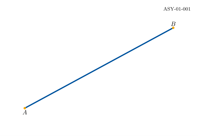
Command or parameter	Meaning
`pair`	A two-component coordinate value.
`--`	Connect positions with a straight segment.
`linewidth(2)`	Specify the stroke in PostScript points.

Complete standalone Asymptote program

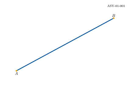
settings.tex="pdflatex";
settings.outformat="pdf";
settings.render=0;
settings.prc=false;
settings.v3d=false;
defaultpen(fontsize(10pt));
pen Blue=rgb(0,84/255.0,159/255.0),Teal=rgb(0,177/255.0,183/255.0);
pen Orange=rgb(246/255.0,168/255.0,0),Green=rgb(87/255.0,171/255.0,39/255.0);
pen Grey=gray(.4),Light=gray(.92),Wash=rgb(232/255.0,241/255.0,250/255.0);
string figureID="ASY-01-001";
size(320,220,IgnoreAspect);
fill(box((0,0),(320,220)),white);
// BEGIN DRAWING
draw((40,45)--(280,175),Blue+linewidth(2));
dot((40,45),Orange+4); dot((280,175),Orange+4);
label("$A$",(40,45),S); label("$B$",(280,175),N);
// END DRAWING
label("ASY-01-001",(310,210),SW,fontsize(8pt));
shipout(figureID);

Download: Asymptote source · SVG figure · Vector PDF · PNG preview

ASY-01-002

Build a polyline

Adding an intermediate point changes a segment into a broken line. The path can be named and reused.

Back to figure overview

Compare with ASY-01-001 · Join two points.

Asymptote drawing

path route=(40,45)--(155,175)--(280,65);
draw(route,Blue+2);
dot(new pair[] {(40,45),(155,175),(280,65)},Orange+4);

Actual output

Build a polyline — ASY-01-002 · Rendered by Asymptote

Asymptote · exit 0

Native compiler log

Compilation completed successfully. No compiler messages were emitted.

Command or parameter	Meaning
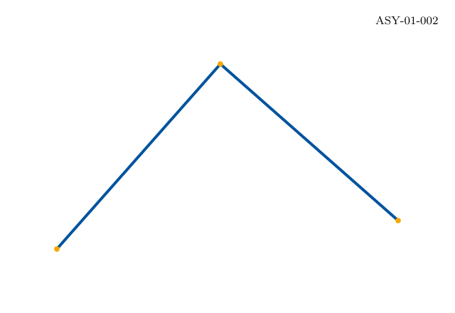
`path`	Store connected geometry as a value.
`new pair[]`	Create an array of points for a single dot call.

Complete standalone Asymptote program

settings.tex="pdflatex";
settings.outformat="pdf";
settings.render=0;
settings.prc=false;
settings.v3d=false;
defaultpen(fontsize(10pt));
pen Blue=rgb(0,84/255.0,159/255.0),Teal=rgb(0,177/255.0,183/255.0);
pen Orange=rgb(246/255.0,168/255.0,0),Green=rgb(87/255.0,171/255.0,39/255.0);
pen Grey=gray(.4),Light=gray(.92),Wash=rgb(232/255.0,241/255.0,250/255.0);
string figureID="ASY-01-002";
size(320,220,IgnoreAspect);
fill(box((0,0),(320,220)),white);
// BEGIN DRAWING
path route=(40,45)--(155,175)--(280,65);
draw(route,Blue+2);
dot(new pair[] {(40,45),(155,175),(280,65)},Orange+4);
// END DRAWING
label("ASY-01-002",(310,210),SW,fontsize(8pt));
shipout(figureID);

Download: Asymptote source · SVG figure · Vector PDF · PNG preview

ASY-01-003

Close and fill a region

cycle closes a path. filldraw gives its interior and boundary independent pens.

Back to figure overview

Asymptote drawing

path triangle=(45,45)--(155,180)--(280,60)--cycle;
filldraw(triangle,Wash,Blue+1.5);

Actual output

Close and fill a region — ASY-01-003 · Rendered by Asymptote

Asymptote · exit 0

Native compiler log

Compilation completed successfully. No compiler messages were emitted.

Command or parameter	Meaning
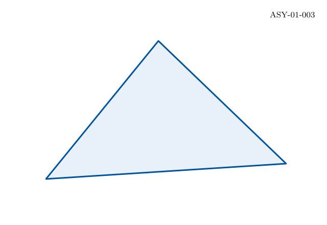
`cycle`	Connect the final point back to the first.
`filldraw`	Fill first, then draw the boundary.

Complete standalone Asymptote program

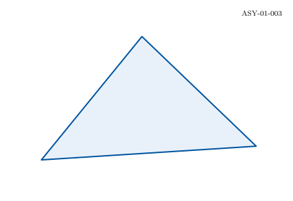
settings.tex="pdflatex";
settings.outformat="pdf";
settings.render=0;
settings.prc=false;
settings.v3d=false;
defaultpen(fontsize(10pt));
pen Blue=rgb(0,84/255.0,159/255.0),Teal=rgb(0,177/255.0,183/255.0);
pen Orange=rgb(246/255.0,168/255.0,0),Green=rgb(87/255.0,171/255.0,39/255.0);
pen Grey=gray(.4),Light=gray(.92),Wash=rgb(232/255.0,241/255.0,250/255.0);
string figureID="ASY-01-003";
size(320,220,IgnoreAspect);
fill(box((0,0),(320,220)),white);
// BEGIN DRAWING
path triangle=(45,45)--(155,180)--(280,60)--cycle;
filldraw(triangle,Wash,Blue+1.5);
// END DRAWING
label("ASY-01-003",(310,210),SW,fontsize(8pt));
shipout(figureID);

Download: Asymptote source · SVG figure · Vector PDF · PNG preview

ASY-01-004

Make coordinates visible

Loops create a reference grid. The named coordinate map separates logical values from positions on the page.

Back to figure overview

Asymptote drawing

real xmin=0,xmax=6,ymin=0,ymax=4;
pair P(real x,real y) {return (45+245*(x-xmin)/(xmax-xmin),35+145*(y-ymin)/(ymax-ymin));}
for(int i=0;i<=4;++i) {
 real x=xmin+i*(xmax-xmin)/4, y=ymin+i*(ymax-ymin)/4;
 draw(P(x,ymin)--P(x,ymax),Light);
 draw(P(xmin,y)--P(xmax,y),Light);
 label(format("$%.3g$",x),P(x,ymin),S);
 label(format("$%.3g$",y),P(xmin,y),W);
}
draw(P(xmin,ymax)--P(xmin,ymin)--P(xmax,ymin),Grey);
draw(P(1,1)--P(5,3),Blue+2);
dot(P(1,1),Orange+4); dot(P(5,3),Orange+4);

Actual output

Make coordinates visible — ASY-01-004 · Rendered by Asymptote

Asymptote · exit 0

Native compiler log

Compilation completed successfully. No compiler messages were emitted.

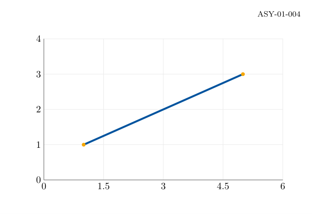
Command or parameter	Meaning
`P(x,y)`	Map data coordinates into the plotting rectangle.
`for`	Repeat drawing operations at computed positions.
`format`	Typeset compact numeric tick labels.

Complete standalone Asymptote program

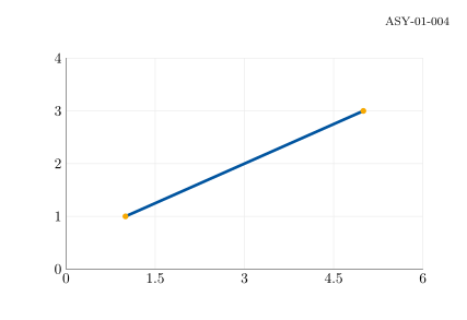
settings.tex="pdflatex";
settings.outformat="pdf";
settings.render=0;
settings.prc=false;
settings.v3d=false;
defaultpen(fontsize(10pt));
pen Blue=rgb(0,84/255.0,159/255.0),Teal=rgb(0,177/255.0,183/255.0);
pen Orange=rgb(246/255.0,168/255.0,0),Green=rgb(87/255.0,171/255.0,39/255.0);
pen Grey=gray(.4),Light=gray(.92),Wash=rgb(232/255.0,241/255.0,250/255.0);
string figureID="ASY-01-004";
size(320,220,IgnoreAspect);
fill(box((0,0),(320,220)),white);
// BEGIN DRAWING
real xmin=0,xmax=6,ymin=0,ymax=4;
pair P(real x,real y) {return (45+245*(x-xmin)/(xmax-xmin),35+145*(y-ymin)/(ymax-ymin));}
for(int i=0;i<=4;++i) {
 real x=xmin+i*(xmax-xmin)/4, y=ymin+i*(ymax-ymin)/4;
 draw(P(x,ymin)--P(x,ymax),Light);
 draw(P(xmin,y)--P(xmax,y),Light);
 label(format("$%.3g$",x),P(x,ymin),S);
 label(format("$%.3g$",y),P(xmin,y),W);
}
draw(P(xmin,ymax)--P(xmin,ymin)--P(xmax,ymin),Grey);
draw(P(1,1)--P(5,3),Blue+2);
dot(P(1,1),Orange+4); dot(P(5,3),Orange+4);
// END DRAWING
label("ASY-01-004",(310,210),SW,fontsize(8pt));
shipout(figureID);

Download: Asymptote source · SVG figure · Vector PDF · PNG preview

ASY-01-005

Draw circles and boxes

Built-in constructors produce reusable paths. Equal radii and independent corner pairs make the geometry explicit.

Back to figure overview

Asymptote drawing

filldraw(circle((85,105),48),Wash,Blue+1.5);
filldraw(box((185,55),(275,155)),Wash,Teal+1.5);
dot((85,105),Orange+4);

Actual output

Draw circles and boxes — ASY-01-005 · Rendered by Asymptote

Asymptote · exit 0

Native compiler log

Compilation completed successfully. No compiler messages were emitted.

Command or parameter	Meaning
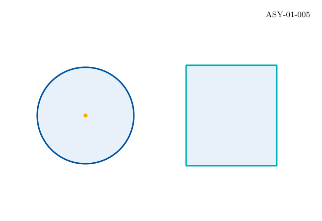
`circle(centre,radius)`	Construct a circle as a path.
`box(lower,upper)`	Construct a rectangular closed path.

Complete standalone Asymptote program

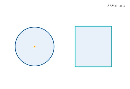
settings.tex="pdflatex";
settings.outformat="pdf";
settings.render=0;
settings.prc=false;
settings.v3d=false;
defaultpen(fontsize(10pt));
pen Blue=rgb(0,84/255.0,159/255.0),Teal=rgb(0,177/255.0,183/255.0);
pen Orange=rgb(246/255.0,168/255.0,0),Green=rgb(87/255.0,171/255.0,39/255.0);
pen Grey=gray(.4),Light=gray(.92),Wash=rgb(232/255.0,241/255.0,250/255.0);
string figureID="ASY-01-005";
size(320,220,IgnoreAspect);
fill(box((0,0),(320,220)),white);
// BEGIN DRAWING
filldraw(circle((85,105),48),Wash,Blue+1.5);
filldraw(box((185,55),(275,155)),Wash,Teal+1.5);
dot((85,105),Orange+4);
// END DRAWING
label("ASY-01-005",(310,210),SW,fontsize(8pt));
shipout(figureID);

Download: Asymptote source · SVG figure · Vector PDF · PNG preview

ASY-01-006

Annotate direction and distance

Arrow and Bars are end markers. Labels use TeX, so mathematical notation and ordinary spaces are typeset together.

Back to figure overview

Asymptote drawing

draw((55,75)--(270,75),Blue+2,Arrow(7));
draw((55,125)--(270,125),Teal,Bars(5));
label("$d=215$ units",(162.5,140),N);
label("direction",(162.5,55),S);

Actual output

Annotate direction and distance — ASY-01-006 · Rendered by Asymptote

Asymptote · exit 0

Native compiler log

Compilation completed successfully. No compiler messages were emitted.

Command or parameter	Meaning
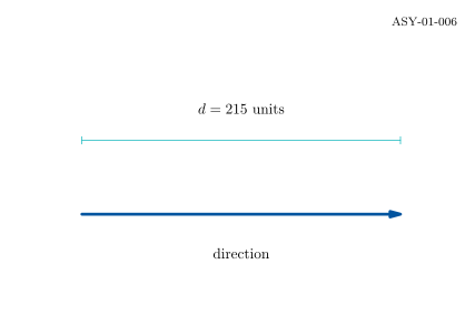
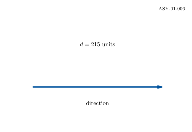
`Arrow(7)`	Attach an arrowhead seven points long.
`Bars(5)`	Attach short perpendicular bars to both ends.
`label`	Typeset text or mathematics at a chosen position.

Complete standalone Asymptote program

settings.tex="pdflatex";
settings.outformat="pdf";
settings.render=0;
settings.prc=false;
settings.v3d=false;
defaultpen(fontsize(10pt));
pen Blue=rgb(0,84/255.0,159/255.0),Teal=rgb(0,177/255.0,183/255.0);
pen Orange=rgb(246/255.0,168/255.0,0),Green=rgb(87/255.0,171/255.0,39/255.0);
pen Grey=gray(.4),Light=gray(.92),Wash=rgb(232/255.0,241/255.0,250/255.0);
string figureID="ASY-01-006";
size(320,220,IgnoreAspect);
fill(box((0,0),(320,220)),white);
// BEGIN DRAWING
draw((55,75)--(270,75),Blue+2,Arrow(7));
draw((55,125)--(270,125),Teal,Bars(5));
label("$d=215$ units",(162.5,140),N);
label("direction",(162.5,55),S);
// END DRAWING
label("ASY-01-006",(310,210),SW,fontsize(8pt));
shipout(figureID);

Download: Asymptote source · SVG figure · Vector PDF · PNG preview

02 · Curves and control points

ASY-02-001

Interpolate a smooth path

Smooth connectors replace the straight segments while preserving the supplied knots. These are interpolation points, not Bezier controls.

Back to figure overview

Compare with ASY-01-002 · Build a polyline.

Asymptote drawing

path p=(40,45)..(155,175)..(280,65);
draw(p,Blue+2);
dot(new pair[] {(40,45),(155,175),(280,65)},Orange+4);

Actual output

Interpolate a smooth path — ASY-02-001 · Rendered by Asymptote

Asymptote · exit 0

Native compiler log

Compilation completed successfully. No compiler messages were emitted.

Command or parameter	Meaning
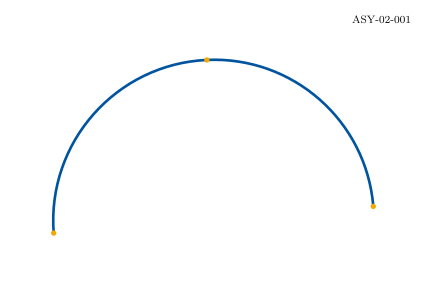
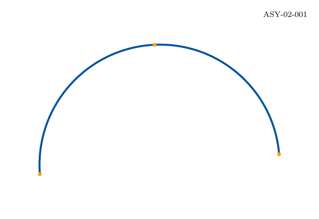
`..`	Ask the Hobby algorithm to choose cubic controls.
`Knots`	The path passes through the supplied points.

Complete standalone Asymptote program

settings.tex="pdflatex";
settings.outformat="pdf";
settings.render=0;
settings.prc=false;
settings.v3d=false;
defaultpen(fontsize(10pt));
pen Blue=rgb(0,84/255.0,159/255.0),Teal=rgb(0,177/255.0,183/255.0);
pen Orange=rgb(246/255.0,168/255.0,0),Green=rgb(87/255.0,171/255.0,39/255.0);
pen Grey=gray(.4),Light=gray(.92),Wash=rgb(232/255.0,241/255.0,250/255.0);
string figureID="ASY-02-001";
size(320,220,IgnoreAspect);
fill(box((0,0),(320,220)),white);
// BEGIN DRAWING
path p=(40,45)..(155,175)..(280,65);
draw(p,Blue+2);
dot(new pair[] {(40,45),(155,175),(280,65)},Orange+4);
// END DRAWING
label("ASY-02-001",(310,210),SW,fontsize(8pt));
shipout(figureID);

Download: Asymptote source · SVG figure · Vector PDF · PNG preview

ASY-02-002

Expose Bezier controls

An explicit cubic separates endpoints from handles. The dashed control polygon shows how the handles influence the curve.

Back to figure overview

Asymptote drawing

pair a=(40,45),b=(65,185),c=(255,185),d=(280,60);
draw(a--b--c--d,Grey+dashed);
draw(a..controls b and c..d,Blue+2);
dot(new pair[] {a,b,c,d},Orange+4);

Actual output

Expose Bezier controls — ASY-02-002 · Rendered by Asymptote

Asymptote · exit 0

Native compiler log

Compilation completed successfully. No compiler messages were emitted.

Command or parameter	Meaning
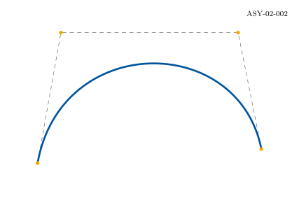
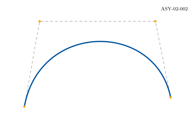
`controls b and c`	Set both handles of one cubic segment.
`Dashed polygon`	Show the relationship between handles and endpoints.

Complete standalone Asymptote program

settings.tex="pdflatex";
settings.outformat="pdf";
settings.render=0;
settings.prc=false;
settings.v3d=false;
defaultpen(fontsize(10pt));
pen Blue=rgb(0,84/255.0,159/255.0),Teal=rgb(0,177/255.0,183/255.0);
pen Orange=rgb(246/255.0,168/255.0,0),Green=rgb(87/255.0,171/255.0,39/255.0);
pen Grey=gray(.4),Light=gray(.92),Wash=rgb(232/255.0,241/255.0,250/255.0);
string figureID="ASY-02-002";
size(320,220,IgnoreAspect);
fill(box((0,0),(320,220)),white);
// BEGIN DRAWING
pair a=(40,45),b=(65,185),c=(255,185),d=(280,60);
draw(a--b--c--d,Grey+dashed);
draw(a..controls b and c..d,Blue+2);
dot(new pair[] {a,b,c,d},Orange+4);
// END DRAWING
label("ASY-02-002",(310,210),SW,fontsize(8pt));
shipout(figureID);

Download: Asymptote source · SVG figure · Vector PDF · PNG preview

ASY-02-003

Constrain endpoint directions

The endpoint directions are vectors. Giving them explicitly controls the tangents while leaving the curve solver to choose handle lengths.

Back to figure overview

Asymptote drawing

path p=(40,45){dir(70)}..{dir(-70)}(280,45);
draw(p,Blue+2);
draw((40,45)--(40,45)+40*dir(70),Teal,Arrow(5));
draw((280,45)-40*dir(-70)--(280,45),Teal,Arrow(5));

Actual output

Constrain endpoint directions — ASY-02-003 · Rendered by Asymptote

Asymptote · exit 0

Native compiler log

Compilation completed successfully. No compiler messages were emitted.

Command or parameter	Meaning
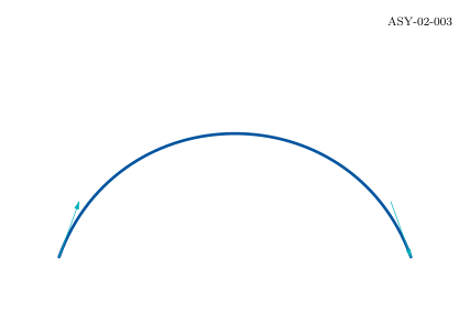
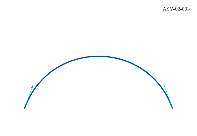
`dir(angle)`	Convert a direction in degrees into a unit pair.
`{direction}`	Constrain a path tangent at a knot.

Complete standalone Asymptote program

settings.tex="pdflatex";
settings.outformat="pdf";
settings.render=0;
settings.prc=false;
settings.v3d=false;
defaultpen(fontsize(10pt));
pen Blue=rgb(0,84/255.0,159/255.0),Teal=rgb(0,177/255.0,183/255.0);
pen Orange=rgb(246/255.0,168/255.0,0),Green=rgb(87/255.0,171/255.0,39/255.0);
pen Grey=gray(.4),Light=gray(.92),Wash=rgb(232/255.0,241/255.0,250/255.0);
string figureID="ASY-02-003";
size(320,220,IgnoreAspect);
fill(box((0,0),(320,220)),white);
// BEGIN DRAWING
path p=(40,45){dir(70)}..{dir(-70)}(280,45);
draw(p,Blue+2);
draw((40,45)--(40,45)+40*dir(70),Teal,Arrow(5));
draw((280,45)-40*dir(-70)--(280,45),Teal,Arrow(5));
// END DRAWING
label("ASY-02-003",(310,210),SW,fontsize(8pt));
shipout(figureID);

Download: Asymptote source · SVG figure · Vector PDF · PNG preview

ASY-02-004

Compare curve tension

Tension changes how tightly a smooth segment approaches its chord. Each row uses identical endpoint directions.

Back to figure overview

Compare with ASY-02-003 · Constrain endpoint directions.

Asymptote drawing

for(int k=0;k<3;++k) {
 real t=1+.8*k;
 path p=(65,40+55*k){dir(55)}..tension t..{dir(-55)}(285,40+55*k);
 draw(p,Blue+1.5);
 label(format("$t=%.1f$",t),(55,40+55*k),W);
}

Actual output

Compare curve tension — ASY-02-004 · Rendered by Asymptote

Asymptote · exit 0

Native compiler log

Compilation completed successfully. No compiler messages were emitted.

Command or parameter	Meaning
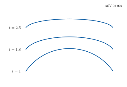
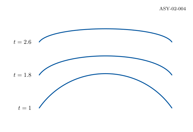
`tension`	Change the relation between handles and the chord.
`Translated rows`	Keep shape comparisons separate.

Complete standalone Asymptote program

settings.tex="pdflatex";
settings.outformat="pdf";
settings.render=0;
settings.prc=false;
settings.v3d=false;
defaultpen(fontsize(10pt));
pen Blue=rgb(0,84/255.0,159/255.0),Teal=rgb(0,177/255.0,183/255.0);
pen Orange=rgb(246/255.0,168/255.0,0),Green=rgb(87/255.0,171/255.0,39/255.0);
pen Grey=gray(.4),Light=gray(.92),Wash=rgb(232/255.0,241/255.0,250/255.0);
string figureID="ASY-02-004";
size(320,220,IgnoreAspect);
fill(box((0,0),(320,220)),white);
// BEGIN DRAWING
for(int k=0;k<3;++k) {
 real t=1+.8*k;
 path p=(65,40+55*k){dir(55)}..tension t..{dir(-55)}(285,40+55*k);
 draw(p,Blue+1.5);
 label(format("$t=%.1f$",t),(55,40+55*k),W);
}
// END DRAWING
label("ASY-02-004",(310,210),SW,fontsize(8pt));
shipout(figureID);

Download: Asymptote source · SVG figure · Vector PDF · PNG preview

ASY-02-005

Sample a path by arc length

Path time is an interpolation parameter; arc length measures physical distance along the path. Equal distance steps create evenly spaced dots.

Back to figure overview

Asymptote drawing

path p=(40,60)..(100,170)..(220,45)..(280,155);
draw(p,Blue+1.5);
real L=arclength(p);
for(int i=0;i<=12;++i)
 dot(point(p,arctime(p,i*L/12)),Orange+4);

Actual output

Sample a path by arc length — ASY-02-005 · Rendered by Asymptote

Asymptote · exit 0

Native compiler log

Compilation completed successfully. No compiler messages were emitted.

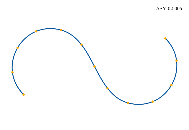
Command or parameter	Meaning
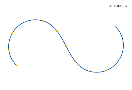
`arclength(p)`	Measure the entire path.
`arctime(p,d)`	Find path time at distance d.
`point(p,t)`	Evaluate a position at path time t.

Complete standalone Asymptote program

settings.tex="pdflatex";
settings.outformat="pdf";
settings.render=0;
settings.prc=false;
settings.v3d=false;
defaultpen(fontsize(10pt));
pen Blue=rgb(0,84/255.0,159/255.0),Teal=rgb(0,177/255.0,183/255.0);
pen Orange=rgb(246/255.0,168/255.0,0),Green=rgb(87/255.0,171/255.0,39/255.0);
pen Grey=gray(.4),Light=gray(.92),Wash=rgb(232/255.0,241/255.0,250/255.0);
string figureID="ASY-02-005";
size(320,220,IgnoreAspect);
fill(box((0,0),(320,220)),white);
// BEGIN DRAWING
path p=(40,60)..(100,170)..(220,45)..(280,155);
draw(p,Blue+1.5);
real L=arclength(p);
for(int i=0;i<=12;++i)
 dot(point(p,arctime(p,i*L/12)),Orange+4);
// END DRAWING
label("ASY-02-005",(310,210),SW,fontsize(8pt));
shipout(figureID);

Download: Asymptote source · SVG figure · Vector PDF · PNG preview

ASY-02-006

Inspect tangents on a closed path

The tangent direction can be evaluated at any path time. Short arrows reveal orientation without replacing the underlying curve.

Back to figure overview

Asymptote drawing

path p=shift(160,105)*xscale(110)*yscale(70)*unitcircle;
filldraw(p,Wash,Blue);
for(int i=0;i<4;++i) {
 real t=i*length(p)/4.0;
 pair q=point(p,t),v=unit(dir(p,t));
 draw(q-18*v--q+18*v,Orange+1.5,Arrow(5));
}

Actual output

Inspect tangents on a closed path — ASY-02-006 · Rendered by Asymptote

Asymptote · exit 0

Native compiler log

Compilation completed successfully. No compiler messages were emitted.

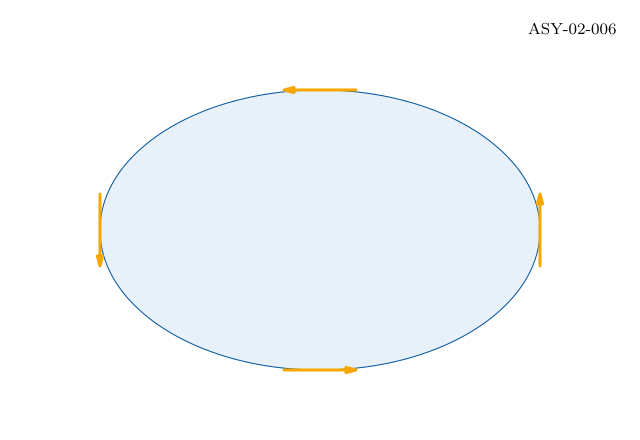
Command or parameter	Meaning
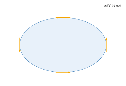
`unitcircle`	A reusable unit-radius circle.
`dir(p,t)`	Evaluate the path tangent.
`unit(vector)`	Normalize a nonzero pair.

Complete standalone Asymptote program

settings.tex="pdflatex";
settings.outformat="pdf";
settings.render=0;
settings.prc=false;
settings.v3d=false;
defaultpen(fontsize(10pt));
pen Blue=rgb(0,84/255.0,159/255.0),Teal=rgb(0,177/255.0,183/255.0);
pen Orange=rgb(246/255.0,168/255.0,0),Green=rgb(87/255.0,171/255.0,39/255.0);
pen Grey=gray(.4),Light=gray(.92),Wash=rgb(232/255.0,241/255.0,250/255.0);
string figureID="ASY-02-006";
size(320,220,IgnoreAspect);
fill(box((0,0),(320,220)),white);
// BEGIN DRAWING
path p=shift(160,105)*xscale(110)*yscale(70)*unitcircle;
filldraw(p,Wash,Blue);
for(int i=0;i<4;++i) {
 real t=i*length(p)/4.0;
 pair q=point(p,t),v=unit(dir(p,t));
 draw(q-18*v--q+18*v,Orange+1.5,Arrow(5));
}
// END DRAWING
label("ASY-02-006",(310,210),SW,fontsize(8pt));
shipout(figureID);

Download: Asymptote source · SVG figure · Vector PDF · PNG preview

03 · Pens, colour and transformations

ASY-03-001

Compare stroke weights

Pen attributes combine by addition. A single path can be drawn repeatedly with independent colour and line width.

Back to figure overview

Asymptote drawing

path wave=(40,0)..(110,25)..(200,-20)..(280,0);
for(int k=0;k<4;++k)
 draw(shift(0,45+42*k)*wave,Blue+linewidth(.4+.8*k));

Actual output

Compare stroke weights — ASY-03-001 · Rendered by Asymptote

Asymptote · exit 0

Native compiler log

Compilation completed successfully. No compiler messages were emitted.

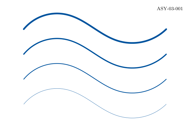
Command or parameter	Meaning
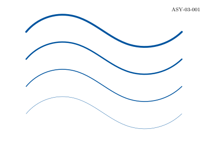
`pen + pen`	Combine colour, width and line-style attributes.
`linewidth`	Choose a width in physical points.

Complete standalone Asymptote program

settings.tex="pdflatex";
settings.outformat="pdf";
settings.render=0;
settings.prc=false;
settings.v3d=false;
defaultpen(fontsize(10pt));
pen Blue=rgb(0,84/255.0,159/255.0),Teal=rgb(0,177/255.0,183/255.0);
pen Orange=rgb(246/255.0,168/255.0,0),Green=rgb(87/255.0,171/255.0,39/255.0);
pen Grey=gray(.4),Light=gray(.92),Wash=rgb(232/255.0,241/255.0,250/255.0);
string figureID="ASY-03-001";
size(320,220,IgnoreAspect);
fill(box((0,0),(320,220)),white);
// BEGIN DRAWING
path wave=(40,0)..(110,25)..(200,-20)..(280,0);
for(int k=0;k<4;++k)
 draw(shift(0,45+42*k)*wave,Blue+linewidth(.4+.8*k));
// END DRAWING
label("ASY-03-001",(310,210),SW,fontsize(8pt));
shipout(figureID);

Download: Asymptote source · SVG figure · Vector PDF · PNG preview

ASY-03-002

Compare dash patterns

The same geometry can carry different dash patterns. These are native vector stroke styles, preserved in every export.

Back to figure overview

Asymptote drawing

draw((40,55)--(280,55),Blue+1.5+dashed);
draw((40,110)--(280,110),Blue+1.5+longdashed);
draw((40,165)--(280,165),Blue+1.5+dashdotted);

Actual output

Compare dash patterns — ASY-03-002 · Rendered by Asymptote

Asymptote · exit 0

Native compiler log

Compilation completed successfully. No compiler messages were emitted.

Command or parameter	Meaning
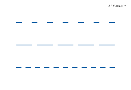
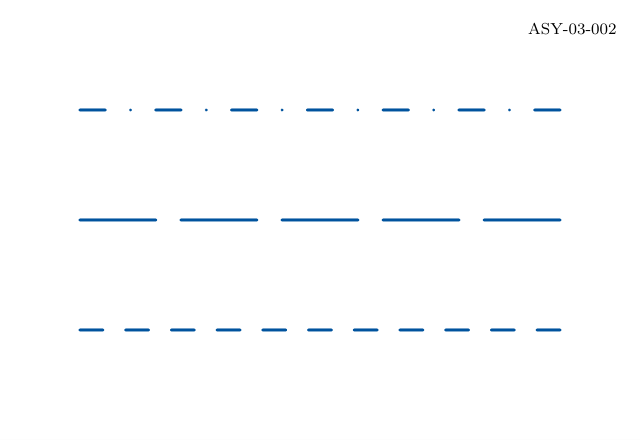
`dashed`	Use the standard short-dash pattern.
`longdashed`	Increase dash length.
`dashdotted`	Alternate dashes and dots.

Complete standalone Asymptote program

settings.tex="pdflatex";
settings.outformat="pdf";
settings.render=0;
settings.prc=false;
settings.v3d=false;
defaultpen(fontsize(10pt));
pen Blue=rgb(0,84/255.0,159/255.0),Teal=rgb(0,177/255.0,183/255.0);
pen Orange=rgb(246/255.0,168/255.0,0),Green=rgb(87/255.0,171/255.0,39/255.0);
pen Grey=gray(.4),Light=gray(.92),Wash=rgb(232/255.0,241/255.0,250/255.0);
string figureID="ASY-03-002";
size(320,220,IgnoreAspect);
fill(box((0,0),(320,220)),white);
// BEGIN DRAWING
draw((40,55)--(280,55),Blue+1.5+dashed);
draw((40,110)--(280,110),Blue+1.5+longdashed);
draw((40,165)--(280,165),Blue+1.5+dashdotted);
// END DRAWING
label("ASY-03-002",(310,210),SW,fontsize(8pt));
shipout(figureID);

Download: Asymptote source · SVG figure · Vector PDF · PNG preview

ASY-03-003

Interpolate a colour ramp

interp blends two pens. The lower strip compares the same blue at different opacities over white.

Back to figure overview

Asymptote drawing

for(int k=0;k<6;++k) {
 real t=k/5.0;
 fill(box((35+43*k,120),(70+43*k,170)),interp(Blue,Teal,t));
 fill(box((35+43*k,45),(70+43*k,95)),Blue+opacity(1-t));
 label(format("%.1f",t),(52+43*k,30));
}

Actual output

Interpolate a colour ramp — ASY-03-003 · Rendered by Asymptote

Asymptote · exit 0

Native compiler log

Compilation completed successfully. No compiler messages were emitted.

Command or parameter	Meaning
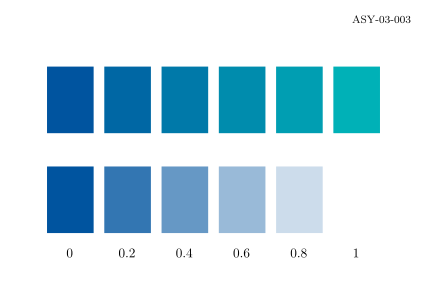
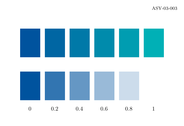
`interp(a,b,t)`	Blend between two colours.
`opacity(alpha)`	Use alpha between zero and one.

Complete standalone Asymptote program

settings.tex="pdflatex";
settings.outformat="pdf";
settings.render=0;
settings.prc=false;
settings.v3d=false;
defaultpen(fontsize(10pt));
pen Blue=rgb(0,84/255.0,159/255.0),Teal=rgb(0,177/255.0,183/255.0);
pen Orange=rgb(246/255.0,168/255.0,0),Green=rgb(87/255.0,171/255.0,39/255.0);
pen Grey=gray(.4),Light=gray(.92),Wash=rgb(232/255.0,241/255.0,250/255.0);
string figureID="ASY-03-003";
size(320,220,IgnoreAspect);
fill(box((0,0),(320,220)),white);
// BEGIN DRAWING
for(int k=0;k<6;++k) {
 real t=k/5.0;
 fill(box((35+43*k,120),(70+43*k,170)),interp(Blue,Teal,t));
 fill(box((35+43*k,45),(70+43*k,95)),Blue+opacity(1-t));
 label(format("%.1f",t),(52+43*k,30));
}
// END DRAWING
label("ASY-03-003",(310,210),SW,fontsize(8pt));
shipout(figureID);

Download: Asymptote source · SVG figure · Vector PDF · PNG preview

ASY-03-004

Transform a reusable motif

A named path can be scaled, rotated and shifted without changing its definition. Here each copy rotates about its own origin.

Back to figure overview

Asymptote drawing

path petal=(0,0)..(25,35)..(50,0)..(25,-12)..cycle;
for(int k=0;k<5;++k)
 filldraw(shift(45+55*k,105)*rotate(25*k)*scale(.65)*petal,
          Wash,interp(Blue,Teal,k/4.0));

Actual output

Transform a reusable motif — ASY-03-004 · Rendered by Asymptote

Asymptote · exit 0

Native compiler log

Compilation completed successfully. No compiler messages were emitted.

Command or parameter	Meaning
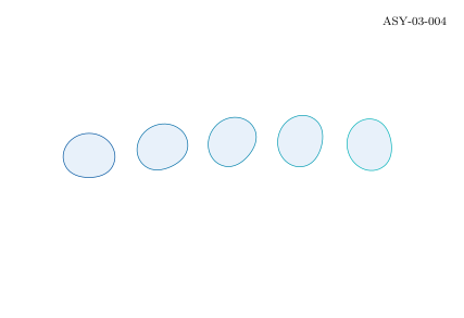
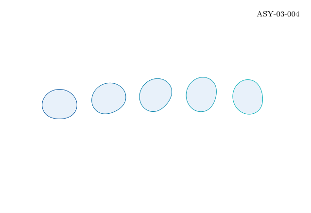
`transform * path`	Apply a transform to stored geometry.
`Rightmost first`	Scale, then rotate, then shift in this expression.

Complete standalone Asymptote program

settings.tex="pdflatex";
settings.outformat="pdf";
settings.render=0;
settings.prc=false;
settings.v3d=false;
defaultpen(fontsize(10pt));
pen Blue=rgb(0,84/255.0,159/255.0),Teal=rgb(0,177/255.0,183/255.0);
pen Orange=rgb(246/255.0,168/255.0,0),Green=rgb(87/255.0,171/255.0,39/255.0);
pen Grey=gray(.4),Light=gray(.92),Wash=rgb(232/255.0,241/255.0,250/255.0);
string figureID="ASY-03-004";
size(320,220,IgnoreAspect);
fill(box((0,0),(320,220)),white);
// BEGIN DRAWING
path petal=(0,0)..(25,35)..(50,0)..(25,-12)..cycle;
for(int k=0;k<5;++k)
 filldraw(shift(45+55*k,105)*rotate(25*k)*scale(.65)*petal,
          Wash,interp(Blue,Teal,k/4.0));
// END DRAWING
label("ASY-03-004",(310,210),SW,fontsize(8pt));
shipout(figureID);

Download: Asymptote source · SVG figure · Vector PDF · PNG preview

ASY-03-005

See why transform order matters

Rotation and translation do not commute. The two copies start from the same asymmetric shape and receive the same two operations in a different order.

Back to figure overview

Compare with ASY-03-004 · Transform a reusable motif.

Asymptote drawing

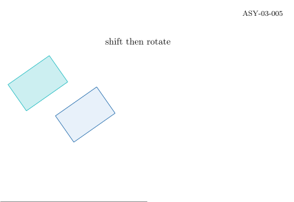
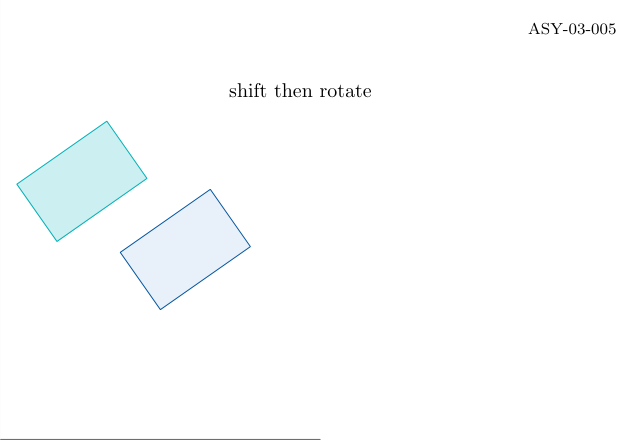
path shape=box((0,0),(55,35));
transform a=shift(80,65)*rotate(35);
transform b=rotate(35)*shift(80,65);
filldraw(a*shape,Wash,Blue);
filldraw(b*shape,interp(white,Teal,.2),Teal);
draw((0,0)--(160,0),Grey);
label("shift then rotate",(150,175));

Actual output

See why transform order matters — ASY-03-005 · Rendered by Asymptote

Asymptote · exit 0

Native compiler log

Compilation completed successfully. No compiler messages were emitted.

Command or parameter	Meaning
`a*b`	Apply b before a.
`Asymmetric shape`	Make the effect of order visible.

Complete standalone Asymptote program

settings.tex="pdflatex";
settings.outformat="pdf";
settings.render=0;
settings.prc=false;
settings.v3d=false;
defaultpen(fontsize(10pt));
pen Blue=rgb(0,84/255.0,159/255.0),Teal=rgb(0,177/255.0,183/255.0);
pen Orange=rgb(246/255.0,168/255.0,0),Green=rgb(87/255.0,171/255.0,39/255.0);
pen Grey=gray(.4),Light=gray(.92),Wash=rgb(232/255.0,241/255.0,250/255.0);
string figureID="ASY-03-005";
size(320,220,IgnoreAspect);
fill(box((0,0),(320,220)),white);
// BEGIN DRAWING
path shape=box((0,0),(55,35));
transform a=shift(80,65)*rotate(35);
transform b=rotate(35)*shift(80,65);
filldraw(a*shape,Wash,Blue);
filldraw(b*shape,interp(white,Teal,.2),Teal);
draw((0,0)--(160,0),Grey);
label("shift then rotate",(150,175));
// END DRAWING
label("ASY-03-005",(310,210),SW,fontsize(8pt));
shipout(figureID);

Download: Asymptote source · SVG figure · Vector PDF · PNG preview

ASY-03-006

Reflect and shear geometry

Reflection changes handedness; shear changes angles while keeping parallel lines parallel. The original supplies a visual baseline.

Back to figure overview

Asymptote drawing

path p=(0,0)--(35,0)--(15,65)--cycle;
filldraw(shift(55,65)*p,Wash,Blue);
filldraw(shift(170,65)*xscale(-1)*p,Wash,Teal);
filldraw(shift(225,65)*slant(.6)*p,Wash,Orange);
label("original",(70,40)); label("reflected",(155,40));
label("sheared",(265,40));

Actual output

Reflect and shear geometry — ASY-03-006 · Rendered by Asymptote

Asymptote · exit 0

Native compiler log

Compilation completed successfully. No compiler messages were emitted.

Command or parameter	Meaning
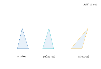
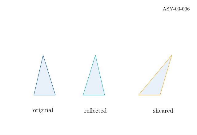
`xscale(-1)`	Reflect the horizontal coordinate.
`slant(.6)`	Apply x = x + 0.6*y.

Complete standalone Asymptote program

settings.tex="pdflatex";
settings.outformat="pdf";
settings.render=0;
settings.prc=false;
settings.v3d=false;
defaultpen(fontsize(10pt));
pen Blue=rgb(0,84/255.0,159/255.0),Teal=rgb(0,177/255.0,183/255.0);
pen Orange=rgb(246/255.0,168/255.0,0),Green=rgb(87/255.0,171/255.0,39/255.0);
pen Grey=gray(.4),Light=gray(.92),Wash=rgb(232/255.0,241/255.0,250/255.0);
string figureID="ASY-03-006";
size(320,220,IgnoreAspect);
fill(box((0,0),(320,220)),white);
// BEGIN DRAWING
path p=(0,0)--(35,0)--(15,65)--cycle;
filldraw(shift(55,65)*p,Wash,Blue);
filldraw(shift(170,65)*xscale(-1)*p,Wash,Teal);
filldraw(shift(225,65)*slant(.6)*p,Wash,Orange);
label("original",(70,40)); label("reflected",(155,40));
label("sheared",(265,40));
// END DRAWING
label("ASY-03-006",(310,210),SW,fontsize(8pt));
shipout(figureID);

Download: Asymptote source · SVG figure · Vector PDF · PNG preview

04 · Programming drawings

ASY-04-001

Use arrays as drawing data

Arrays separate values from their visual encoding. The loop uses each value as a radius and as a label.

Back to figure overview

Asymptote drawing

real[] radius={12,18,25,32,22};
for(int i=0;i<radius.length;++i) {
 pair centre=(45+57*i,105);
 filldraw(circle(centre,radius[i]),Wash,Blue);
 label(format("$r=%.0f$",radius[i]),centre+(0,-48));
}

Actual output

Use arrays as drawing data — ASY-04-001 · Rendered by Asymptote

Asymptote · exit 0

Native compiler log

Compilation completed successfully. No compiler messages were emitted.

Command or parameter	Meaning
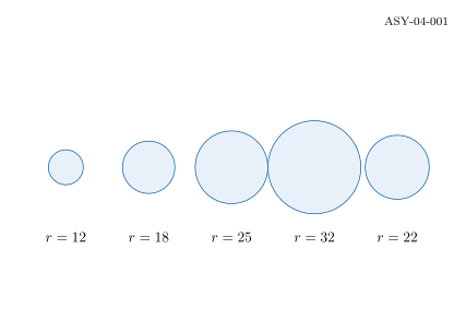
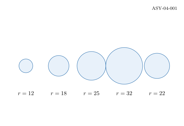
`real[]`	Store numeric data in a typed array.
`.length`	Read the number of entries.
`Array indexing`	Asymptote arrays start at zero.

Complete standalone Asymptote program

settings.tex="pdflatex";
settings.outformat="pdf";
settings.render=0;
settings.prc=false;
settings.v3d=false;
defaultpen(fontsize(10pt));
pen Blue=rgb(0,84/255.0,159/255.0),Teal=rgb(0,177/255.0,183/255.0);
pen Orange=rgb(246/255.0,168/255.0,0),Green=rgb(87/255.0,171/255.0,39/255.0);
pen Grey=gray(.4),Light=gray(.92),Wash=rgb(232/255.0,241/255.0,250/255.0);
string figureID="ASY-04-001";
size(320,220,IgnoreAspect);
fill(box((0,0),(320,220)),white);
// BEGIN DRAWING
real[] radius={12,18,25,32,22};
for(int i=0;i<radius.length;++i) {
 pair centre=(45+57*i,105);
 filldraw(circle(centre,radius[i]),Wash,Blue);
 label(format("$r=%.0f$",radius[i]),centre+(0,-48));
}
// END DRAWING
label("ASY-04-001",(310,210),SW,fontsize(8pt));
shipout(figureID);

Download: Asymptote source · SVG figure · Vector PDF · PNG preview

ASY-04-002

Write a pair-valued function

A function encapsulates a coordinate calculation. Calling it with different arguments builds a consistent family of marks.

Back to figure overview

Asymptote drawing

pair place(real t) {return (160,105)+(95*cos(t),65*sin(t));}
for(int i=0;i<12;++i) {
 pair q=place(2*pi*i/12);
 draw((160,105)--q,Light);
 dot(q,interp(Blue,Teal,i/11.0)+5);
}

Actual output

Write a pair-valued function — ASY-04-002 · Rendered by Asymptote

Asymptote · exit 0

Native compiler log

Compilation completed successfully. No compiler messages were emitted.

Command or parameter	Meaning
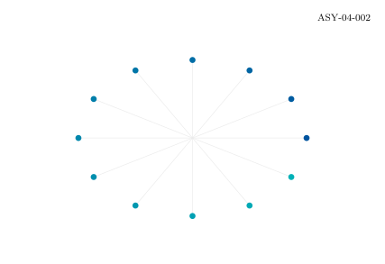
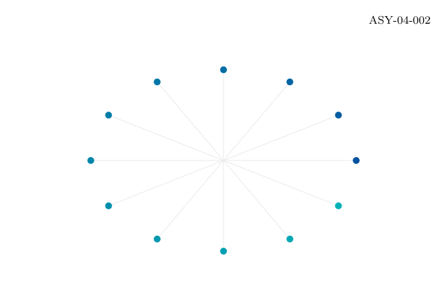
`pair place(real t)`	Return a coordinate from a real parameter.
`sin / cos`	Trigonometric function arguments are radians.

Complete standalone Asymptote program

settings.tex="pdflatex";
settings.outformat="pdf";
settings.render=0;
settings.prc=false;
settings.v3d=false;
defaultpen(fontsize(10pt));
pen Blue=rgb(0,84/255.0,159/255.0),Teal=rgb(0,177/255.0,183/255.0);
pen Orange=rgb(246/255.0,168/255.0,0),Green=rgb(87/255.0,171/255.0,39/255.0);
pen Grey=gray(.4),Light=gray(.92),Wash=rgb(232/255.0,241/255.0,250/255.0);
string figureID="ASY-04-002";
size(320,220,IgnoreAspect);
fill(box((0,0),(320,220)),white);
// BEGIN DRAWING
pair place(real t) {return (160,105)+(95*cos(t),65*sin(t));}
for(int i=0;i<12;++i) {
 pair q=place(2*pi*i/12);
 draw((160,105)--q,Light);
 dot(q,interp(Blue,Teal,i/11.0)+5);
}
// END DRAWING
label("ASY-04-002",(310,210),SW,fontsize(8pt));
shipout(figureID);

Download: Asymptote source · SVG figure · Vector PDF · PNG preview

ASY-04-003

Make a drawing procedure

A procedure can receive geometry and styling. Reusing it keeps the diagram consistent while leaving each call easy to read.

Back to figure overview

Asymptote drawing

void node(string name,pair p,pen colour) {
 filldraw(circle(p,25),Wash,colour+1.5);
 label(name,p);
}
node("input",(60,105),Blue);
node("model",(160,105),Teal);
node("output",(260,105),Blue);
draw((85,105)--(135,105),Grey,Arrow(5));
draw((185,105)--(235,105),Grey,Arrow(5));

Actual output

Make a drawing procedure — ASY-04-003 · Rendered by Asymptote

Asymptote · exit 0

Native compiler log

Compilation completed successfully. No compiler messages were emitted.

Command or parameter	Meaning
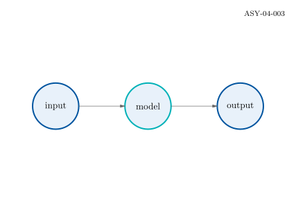
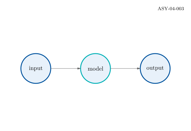
`void function`	Perform drawing operations without returning a value.
`Typed parameters`	Make text, position and colour explicit inputs.

Complete standalone Asymptote program

settings.tex="pdflatex";
settings.outformat="pdf";
settings.render=0;
settings.prc=false;
settings.v3d=false;
defaultpen(fontsize(10pt));
pen Blue=rgb(0,84/255.0,159/255.0),Teal=rgb(0,177/255.0,183/255.0);
pen Orange=rgb(246/255.0,168/255.0,0),Green=rgb(87/255.0,171/255.0,39/255.0);
pen Grey=gray(.4),Light=gray(.92),Wash=rgb(232/255.0,241/255.0,250/255.0);
string figureID="ASY-04-003";
size(320,220,IgnoreAspect);
fill(box((0,0),(320,220)),white);
// BEGIN DRAWING
void node(string name,pair p,pen colour) {
 filldraw(circle(p,25),Wash,colour+1.5);
 label(name,p);
}
node("input",(60,105),Blue);
node("model",(160,105),Teal);
node("output",(260,105),Blue);
draw((85,105)--(135,105),Grey,Arrow(5));
draw((185,105)--(235,105),Grey,Arrow(5));
// END DRAWING
label("ASY-04-003",(310,210),SW,fontsize(8pt));
shipout(figureID);

Download: Asymptote source · SVG figure · Vector PDF · PNG preview

ASY-04-004

Use a structure for related values

A struct groups a name, location and magnitude. The data remain associated as the loop chooses positions, sizes and labels.

Back to figure overview

Asymptote drawing

struct Observation {string name; pair p; real value;}
Observation[] samples=new Observation[3];
for(int i=0;i<3;++i) {
 samples[i]=new Observation;
 samples[i].name="sample "+(string)(i+1);
 samples[i].p=(65+95*i,105);
 samples[i].value=12+8*i;
 filldraw(circle(samples[i].p,samples[i].value),Wash,Blue);
 label(samples[i].name,samples[i].p+(0,-50));
}

Actual output

Use a structure for related values — ASY-04-004 · Rendered by Asymptote

Asymptote · exit 0

Native compiler log

Compilation completed successfully. No compiler messages were emitted.

Command or parameter	Meaning
`struct`	Group related fields under one type.
`new Observation`	Allocate a value before assigning its fields.

Complete standalone Asymptote program

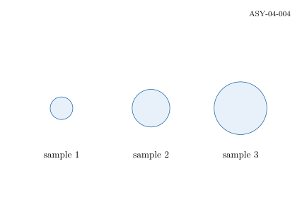
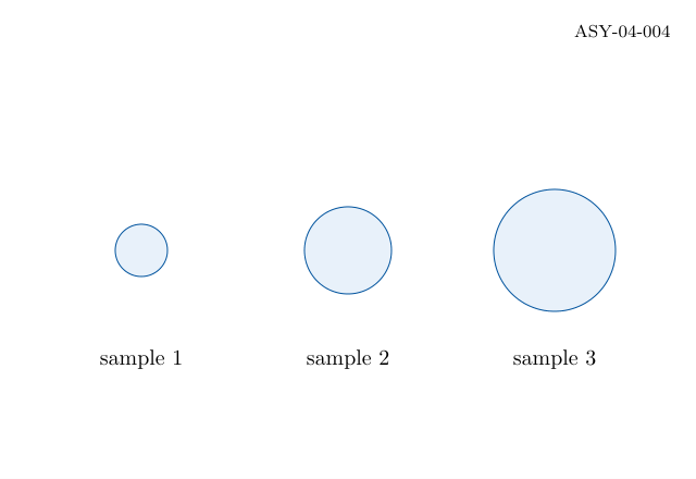
settings.tex="pdflatex";
settings.outformat="pdf";
settings.render=0;
settings.prc=false;
settings.v3d=false;
defaultpen(fontsize(10pt));
pen Blue=rgb(0,84/255.0,159/255.0),Teal=rgb(0,177/255.0,183/255.0);
pen Orange=rgb(246/255.0,168/255.0,0),Green=rgb(87/255.0,171/255.0,39/255.0);
pen Grey=gray(.4),Light=gray(.92),Wash=rgb(232/255.0,241/255.0,250/255.0);
string figureID="ASY-04-004";
size(320,220,IgnoreAspect);
fill(box((0,0),(320,220)),white);
// BEGIN DRAWING
struct Observation {string name; pair p; real value;}
Observation[] samples=new Observation[3];
for(int i=0;i<3;++i) {
 samples[i]=new Observation;
 samples[i].name="sample "+(string)(i+1);
 samples[i].p=(65+95*i,105);
 samples[i].value=12+8*i;
 filldraw(circle(samples[i].p,samples[i].value),Wash,Blue);
 label(samples[i].name,samples[i].p+(0,-50));
}
// END DRAWING
label("ASY-04-004",(310,210),SW,fontsize(8pt));
shipout(figureID);

Download: Asymptote source · SVG figure · Vector PDF · PNG preview

ASY-04-005

Distinguish a branch from a loop

A conditional selects the style of each element. Here positive and negative values share a zero baseline.

Back to figure overview

Asymptote drawing

real[] value={-2,3,1,-4,5,2};
draw((30,105)--(295,105),Grey);
for(int i=0;i<value.length;++i) {
 pair a=(40+42*i,105),b=a+(30,14*value[i]);
 fill(box((a.x,min(a.y,b.y)),(b.x,max(a.y,b.y))),
      value[i]>=0 ? Blue : Orange);
}

Actual output

Distinguish a branch from a loop — ASY-04-005 · Rendered by Asymptote

Asymptote · exit 0

Native compiler log

Compilation completed successfully. No compiler messages were emitted.

Command or parameter	Meaning
`condition ? a : b`	Select one pen from a Boolean condition.
`min / max`	Order rectangle corners for either sign.

Complete standalone Asymptote program

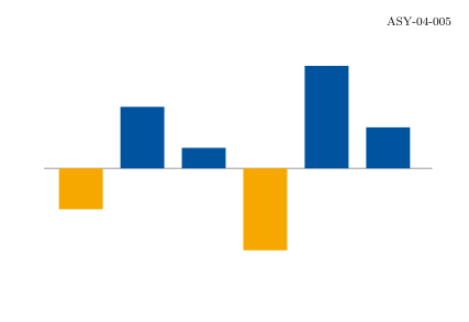
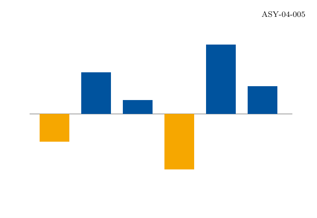
settings.tex="pdflatex";
settings.outformat="pdf";
settings.render=0;
settings.prc=false;
settings.v3d=false;
defaultpen(fontsize(10pt));
pen Blue=rgb(0,84/255.0,159/255.0),Teal=rgb(0,177/255.0,183/255.0);
pen Orange=rgb(246/255.0,168/255.0,0),Green=rgb(87/255.0,171/255.0,39/255.0);
pen Grey=gray(.4),Light=gray(.92),Wash=rgb(232/255.0,241/255.0,250/255.0);
string figureID="ASY-04-005";
size(320,220,IgnoreAspect);
fill(box((0,0),(320,220)),white);
// BEGIN DRAWING
real[] value={-2,3,1,-4,5,2};
draw((30,105)--(295,105),Grey);
for(int i=0;i<value.length;++i) {
 pair a=(40+42*i,105),b=a+(30,14*value[i]);
 fill(box((a.x,min(a.y,b.y)),(b.x,max(a.y,b.y))),
      value[i]>=0 ? Blue : Orange);
}
// END DRAWING
label("ASY-04-005",(310,210),SW,fontsize(8pt));
shipout(figureID);

Download: Asymptote source · SVG figure · Vector PDF · PNG preview

ASY-04-006

Check a numeric calculation in the program

Compute a discrete centroid, draw it and record the result in the compiler output. A numerical check complements the picture.

Back to figure overview

Asymptote drawing

pair[] points={(45,45),(270,60),(155,175)};
pair centre=(0,0);
for(pair p:points) centre+=p/points.length;
draw(points[0]--points[1]--points[2]--cycle,Blue+1.5);
dot(centre,Orange+7);
label("centroid",centre,N);
write("check: centroid="+(string)centre);

Actual output

Check a numeric calculation in the program — ASY-04-006 · Rendered by Asymptote

Asymptote · exit 0

Native compiler log

Standard output

check: centroid=(156.666666666667,93.3333333333333)

Command or parameter	Meaning
`for(pair p:points)`	Iterate over array elements.
`Vector arithmetic`	Average the coordinates component by component.
`write`	Record a value in captured standard output.

Complete standalone Asymptote program

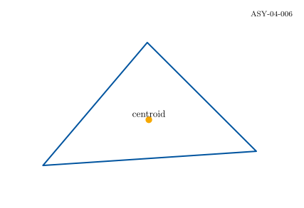
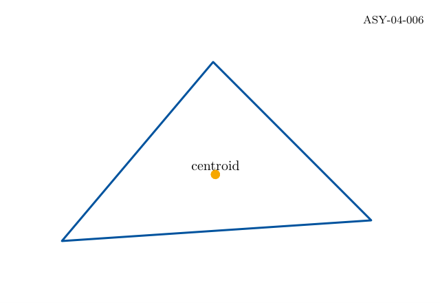
settings.tex="pdflatex";
settings.outformat="pdf";
settings.render=0;
settings.prc=false;
settings.v3d=false;
defaultpen(fontsize(10pt));
pen Blue=rgb(0,84/255.0,159/255.0),Teal=rgb(0,177/255.0,183/255.0);
pen Orange=rgb(246/255.0,168/255.0,0),Green=rgb(87/255.0,171/255.0,39/255.0);
pen Grey=gray(.4),Light=gray(.92),Wash=rgb(232/255.0,241/255.0,250/255.0);
string figureID="ASY-04-006";
size(320,220,IgnoreAspect);
fill(box((0,0),(320,220)),white);
// BEGIN DRAWING
pair[] points={(45,45),(270,60),(155,175)};
pair centre=(0,0);
for(pair p:points) centre+=p/points.length;
draw(points[0]--points[1]--points[2]--cycle,Blue+1.5);
dot(centre,Orange+7);
label("centroid",centre,N);
write("check: centroid="+(string)centre);
// END DRAWING
label("ASY-04-006",(310,210),SW,fontsize(8pt));
shipout(figureID);

Download: Asymptote source · SVG figure · Vector PDF · PNG preview

05 · Functions and parametric plots

ASY-05-001

Plot a function and its derivative

The graph module samples mathematical functions in their own coordinates. Sine and its derivative cosine share labelled axes and distinct pens.

Back to figure overview

Asymptote drawing

import graph;
draw(graph(sin,0,2*pi,200),Blue+1.5);
draw(graph(cos,0,2*pi,200),Teal+1.5+dashed);
xaxis("$x$",BottomTop,Ticks); yaxis("$y$",LeftRight,Ticks);
label("$\sin x$",(1,1.15),Blue);
label("$\cos x$",(5,1.15),Teal);

Actual output

Plot a function and its derivative — ASY-05-001 · Rendered by Asymptote

Asymptote · exit 0

Native compiler log

Compilation completed successfully. No compiler messages were emitted.

Command or parameter	Meaning
`graph(f,a,b,n)`	Sample n subdivisions over a real interval.
`BottomTop / LeftRight`	Draw both sides of the plotting frame.
`Ticks`	Use automatically chosen tick labels.

Complete standalone Asymptote program

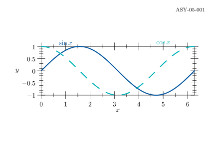
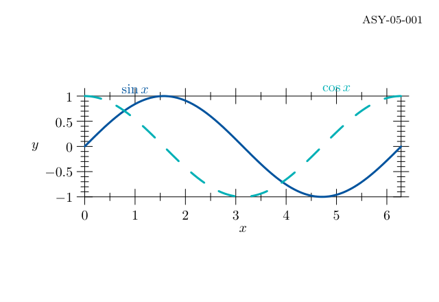
settings.tex="pdflatex";
settings.outformat="pdf";
settings.render=0;
settings.prc=false;
settings.v3d=false;
defaultpen(fontsize(10pt));
pen Blue=rgb(0,84/255.0,159/255.0),Teal=rgb(0,177/255.0,183/255.0);
pen Orange=rgb(246/255.0,168/255.0,0),Green=rgb(87/255.0,171/255.0,39/255.0);
pen Grey=gray(.4),Light=gray(.92),Wash=rgb(232/255.0,241/255.0,250/255.0);
string figureID="ASY-05-001";
size(270,165);
// BEGIN DRAWING
import graph;
draw(graph(sin,0,2*pi,200),Blue+1.5);
draw(graph(cos,0,2*pi,200),Teal+1.5+dashed);
xaxis("$x$",BottomTop,Ticks); yaxis("$y$",LeftRight,Ticks);
label("$\sin x$",(1,1.15),Blue);
label("$\cos x$",(5,1.15),Teal);
// END DRAWING
picture drawing=currentpicture;
currentpicture=new picture;
size(320,220,IgnoreAspect);
fill(box((0,0),(320,220)),white);
add(drawing.fit(),(160,105),align=0);
label("ASY-05-001",(310,210),SW,fontsize(8pt));
shipout(figureID);

Download: Asymptote source · SVG figure · Vector PDF · PNG preview

ASY-05-002

Fill the area between functions

Two sampled functions bound a closed region. Reversing the lower path closes the area in the correct order.

Back to figure overview

Asymptote drawing

import graph;
real f(real x) {return 1+.6*sin(pi*x);}
real g(real x) {return .2-.3*sin(pi*x);}
path a=graph(f,0,1,100),b=graph(g,0,1,100);
fill(a--reverse(b)--cycle,Wash);
draw(a,Blue+1.5); draw(b,Teal+1.5);
xaxis("$x$",Bottom,Ticks); yaxis("$y$",Left,Ticks);

Actual output

Fill the area between functions — ASY-05-002 · Rendered by Asymptote

Asymptote · exit 0

Native compiler log

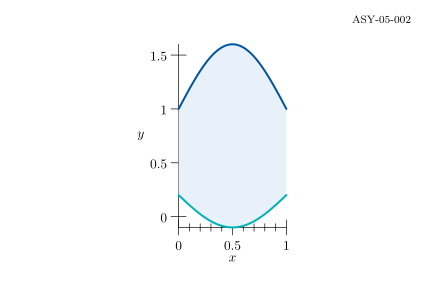
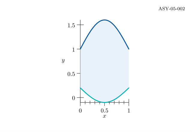
Compilation completed successfully. No compiler messages were emitted.

Command or parameter	Meaning
`reverse(b)`	Traverse the lower boundary in the opposite direction.
`Closed region`	Join both ends before filling.

Complete standalone Asymptote program

settings.tex="pdflatex";
settings.outformat="pdf";
settings.render=0;
settings.prc=false;
settings.v3d=false;
defaultpen(fontsize(10pt));
pen Blue=rgb(0,84/255.0,159/255.0),Teal=rgb(0,177/255.0,183/255.0);
pen Orange=rgb(246/255.0,168/255.0,0),Green=rgb(87/255.0,171/255.0,39/255.0);
pen Grey=gray(.4),Light=gray(.92),Wash=rgb(232/255.0,241/255.0,250/255.0);
string figureID="ASY-05-002";
size(270,165);
// BEGIN DRAWING
import graph;
real f(real x) {return 1+.6*sin(pi*x);}
real g(real x) {return .2-.3*sin(pi*x);}
path a=graph(f,0,1,100),b=graph(g,0,1,100);
fill(a--reverse(b)--cycle,Wash);
draw(a,Blue+1.5); draw(b,Teal+1.5);
xaxis("$x$",Bottom,Ticks); yaxis("$y$",Left,Ticks);
// END DRAWING
picture drawing=currentpicture;
currentpicture=new picture;
size(320,220,IgnoreAspect);
fill(box((0,0),(320,220)),white);
add(drawing.fit(),(160,105),align=0);
label("ASY-05-002",(310,210),SW,fontsize(8pt));
shipout(figureID);

Download: Asymptote source · SVG figure · Vector PDF · PNG preview

ASY-05-003

Choose logarithmic coordinates

Logarithmic scaling makes equal ratios occupy equal distances. Every y value in this example is strictly positive.

Back to figure overview

Asymptote drawing

import graph;
scale(Linear,Log);
real f(real x) {return exp(x);}
draw(graph(f,0,5,100),Blue+1.5);
xaxis("$x$",BottomTop,Ticks);
yaxis("$e^x$",LeftRight,Ticks);

Actual output

Choose logarithmic coordinates — ASY-05-003 · Rendered by Asymptote

Asymptote · exit 0

Native compiler log

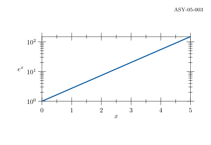
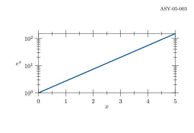
Compilation completed successfully. No compiler messages were emitted.

Command or parameter	Meaning
`scale(Linear,Log)`	Keep x linear and make y logarithmic.
`Positive y`	Logarithms require positive data.

Complete standalone Asymptote program

settings.tex="pdflatex";
settings.outformat="pdf";
settings.render=0;
settings.prc=false;
settings.v3d=false;
defaultpen(fontsize(10pt));
pen Blue=rgb(0,84/255.0,159/255.0),Teal=rgb(0,177/255.0,183/255.0);
pen Orange=rgb(246/255.0,168/255.0,0),Green=rgb(87/255.0,171/255.0,39/255.0);
pen Grey=gray(.4),Light=gray(.92),Wash=rgb(232/255.0,241/255.0,250/255.0);
string figureID="ASY-05-003";
size(270,165);
// BEGIN DRAWING
import graph;
scale(Linear,Log);
real f(real x) {return exp(x);}
draw(graph(f,0,5,100),Blue+1.5);
xaxis("$x$",BottomTop,Ticks);
yaxis("$e^x$",LeftRight,Ticks);
// END DRAWING
picture drawing=currentpicture;
currentpicture=new picture;
size(320,220,IgnoreAspect);
fill(box((0,0),(320,220)),white);
add(drawing.fit(),(160,105),align=0);
label("ASY-05-003",(310,210),SW,fontsize(8pt));
shipout(figureID);

Download: Asymptote source · SVG figure · Vector PDF · PNG preview

ASY-05-004

Draw a parametric Lissajous curve

A pair-valued function defines both coordinates from one parameter. The two frequencies control the lobes of the closed trajectory.

Back to figure overview

Asymptote drawing

import graph;
pair f(real t) {return (sin(3*t),cos(2*t));}
draw(graph(f,0,2*pi,400),Blue+1.5);
xaxis("$x$",BottomTop,Ticks); yaxis("$y$",LeftRight,Ticks);

Actual output

Draw a parametric Lissajous curve — ASY-05-004 · Rendered by Asymptote

Asymptote · exit 0

Native compiler log

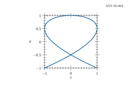
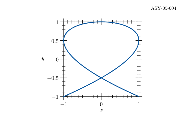
Compilation completed successfully. No compiler messages were emitted.

Command or parameter	Meaning
`pair f(t)`	Return both x and y coordinates.
`0 to 2*pi`	Trace a full period for these integer frequencies.

Complete standalone Asymptote program

settings.tex="pdflatex";
settings.outformat="pdf";
settings.render=0;
settings.prc=false;
settings.v3d=false;
defaultpen(fontsize(10pt));
pen Blue=rgb(0,84/255.0,159/255.0),Teal=rgb(0,177/255.0,183/255.0);
pen Orange=rgb(246/255.0,168/255.0,0),Green=rgb(87/255.0,171/255.0,39/255.0);
pen Grey=gray(.4),Light=gray(.92),Wash=rgb(232/255.0,241/255.0,250/255.0);
string figureID="ASY-05-004";
size(270,165);
// BEGIN DRAWING
import graph;
pair f(real t) {return (sin(3*t),cos(2*t));}
draw(graph(f,0,2*pi,400),Blue+1.5);
xaxis("$x$",BottomTop,Ticks); yaxis("$y$",LeftRight,Ticks);
// END DRAWING
picture drawing=currentpicture;
currentpicture=new picture;
size(320,220,IgnoreAspect);
fill(box((0,0),(320,220)),white);
add(drawing.fit(),(160,105),align=0);
label("ASY-05-004",(310,210),SW,fontsize(8pt));
shipout(figureID);

Download: Asymptote source · SVG figure · Vector PDF · PNG preview

ASY-05-005

Draw a five-petal polar rose

polargraph maps radius and angle into Cartesian coordinates. Negative radii are allowed and are part of the rose construction.

Back to figure overview

Asymptote drawing

import graph;
real r(real t) {return cos(5*t);}
path p=polargraph(r,0,pi,500);
filldraw(p--cycle,Wash,Blue+1.5);
xaxis("$x$",BottomTop,Ticks); yaxis("$y$",LeftRight,Ticks);

Actual output

Draw a five-petal polar rose — ASY-05-005 · Rendered by Asymptote

Asymptote · exit 0

Native compiler log

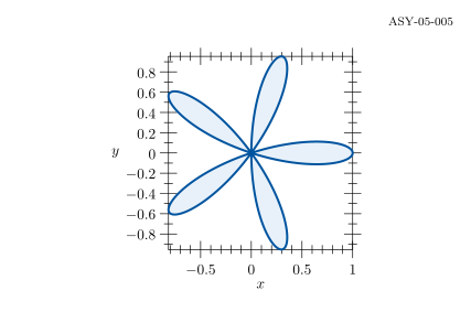
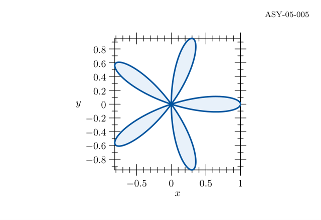
Compilation completed successfully. No compiler messages were emitted.

Command or parameter	Meaning
`polargraph`	Convert a radial function into a path.
`Odd frequency`	A pi-length interval traces the five petals once.

Complete standalone Asymptote program

settings.tex="pdflatex";
settings.outformat="pdf";
settings.render=0;
settings.prc=false;
settings.v3d=false;
defaultpen(fontsize(10pt));
pen Blue=rgb(0,84/255.0,159/255.0),Teal=rgb(0,177/255.0,183/255.0);
pen Orange=rgb(246/255.0,168/255.0,0),Green=rgb(87/255.0,171/255.0,39/255.0);
pen Grey=gray(.4),Light=gray(.92),Wash=rgb(232/255.0,241/255.0,250/255.0);
string figureID="ASY-05-005";
size(270,165);
// BEGIN DRAWING
import graph;
real r(real t) {return cos(5*t);}
path p=polargraph(r,0,pi,500);
filldraw(p--cycle,Wash,Blue+1.5);
xaxis("$x$",BottomTop,Ticks); yaxis("$y$",LeftRight,Ticks);
// END DRAWING
picture drawing=currentpicture;
currentpicture=new picture;
size(320,220,IgnoreAspect);
fill(box((0,0),(320,220)),white);
add(drawing.fit(),(160,105),align=0);
label("ASY-05-005",(310,210),SW,fontsize(8pt));
shipout(figureID);

Download: Asymptote source · SVG figure · Vector PDF · PNG preview

ASY-05-006

Estimate an integral with trapezoids

Numerical integration sums the average height of adjacent samples. The printed estimate is checked independently during tour validation.

Back to figure overview

Asymptote drawing

real xmin=0,xmax=4,ymin=0,ymax=2;
pair P(real x,real y) {return (45+245*(x-xmin)/(xmax-xmin),35+145*(y-ymin)/(ymax-ymin));}
for(int i=0;i<=4;++i) {
 real x=xmin+i*(xmax-xmin)/4, y=ymin+i*(ymax-ymin)/4;
 draw(P(x,ymin)--P(x,ymax),Light);
 draw(P(xmin,y)--P(xmax,y),Light);
 label(format("$%.3g$",x),P(x,ymin),S);
 label(format("$%.3g$",y),P(xmin,y),W);
}
draw(P(xmin,ymax)--P(xmin,ymin)--P(xmax,ymin),Grey);
import graph;
real f(real x) {return 1+.5*cos(pi*x/2);}
pair q(real x) {return P(x,f(x));}
path p=graph(q,0,4,160);
fill(p--P(4,0)--P(0,0)--cycle,Wash); draw(p,Blue+1.5);
int n=200; real h=4.0/n,area=0;
for(int i=0;i<n;++i) area+=h*(f(i*h)+f((i+1)*h))/2;
label(format("Area $\approx %.3f$",area),(165,195));
write("check: area="+(string)area);

Actual output

Estimate an integral with trapezoids — ASY-05-006 · Rendered by Asymptote

Asymptote · exit 0

Native compiler log

Standard output

check: area=4

Command or parameter	Meaning
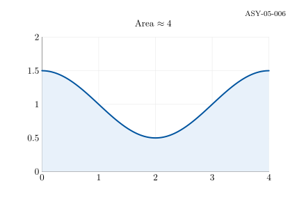
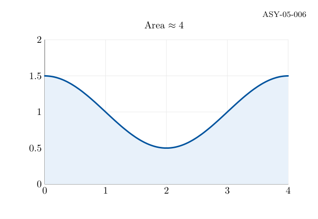
`Trapezoid rule`	Average adjacent sample heights and multiply by step width.
`n=200`	Set the number of integration intervals.

Complete standalone Asymptote program

settings.tex="pdflatex";
settings.outformat="pdf";
settings.render=0;
settings.prc=false;
settings.v3d=false;
defaultpen(fontsize(10pt));
pen Blue=rgb(0,84/255.0,159/255.0),Teal=rgb(0,177/255.0,183/255.0);
pen Orange=rgb(246/255.0,168/255.0,0),Green=rgb(87/255.0,171/255.0,39/255.0);
pen Grey=gray(.4),Light=gray(.92),Wash=rgb(232/255.0,241/255.0,250/255.0);
string figureID="ASY-05-006";
size(320,220,IgnoreAspect);
fill(box((0,0),(320,220)),white);
// BEGIN DRAWING
real xmin=0,xmax=4,ymin=0,ymax=2;
pair P(real x,real y) {return (45+245*(x-xmin)/(xmax-xmin),35+145*(y-ymin)/(ymax-ymin));}
for(int i=0;i<=4;++i) {
 real x=xmin+i*(xmax-xmin)/4, y=ymin+i*(ymax-ymin)/4;
 draw(P(x,ymin)--P(x,ymax),Light);
 draw(P(xmin,y)--P(xmax,y),Light);
 label(format("$%.3g$",x),P(x,ymin),S);
 label(format("$%.3g$",y),P(xmin,y),W);
}
draw(P(xmin,ymax)--P(xmin,ymin)--P(xmax,ymin),Grey);
import graph;
real f(real x) {return 1+.5*cos(pi*x/2);}
pair q(real x) {return P(x,f(x));}
path p=graph(q,0,4,160);
fill(p--P(4,0)--P(0,0)--cycle,Wash); draw(p,Blue+1.5);
int n=200; real h=4.0/n,area=0;
for(int i=0;i<n;++i) area+=h*(f(i*h)+f((i+1)*h))/2;
label(format("Area $\approx %.3f$",area),(165,195));
write("check: area="+(string)area);
// END DRAWING
label("ASY-05-006",(310,210),SW,fontsize(8pt));
shipout(figureID);

Download: Asymptote source · SVG figure · Vector PDF · PNG preview

06 · Data and statistical graphics

ASY-06-001

Build bars from an array

The category values control bar height. A zero baseline keeps lengths proportional to values.

Back to figure overview

Asymptote drawing

real xmin=0,xmax=6,ymin=0,ymax=10;
pair P(real x,real y) {return (45+245*(x-xmin)/(xmax-xmin),35+145*(y-ymin)/(ymax-ymin));}
for(int i=0;i<=4;++i) {
 real x=xmin+i*(xmax-xmin)/4, y=ymin+i*(ymax-ymin)/4;
 draw(P(x,ymin)--P(x,ymax),Light);
 draw(P(xmin,y)--P(xmax,y),Light);
 label(format("$%.3g$",x),P(x,ymin),S);
 label(format("$%.3g$",y),P(xmin,y),W);
}
draw(P(xmin,ymax)--P(xmin,ymin)--P(xmax,ymin),Grey);
real[] v={3,7,5,9,6,8};
for(int i=0;i<v.length;++i) {
 fill(box(P(i+.18,0),P(i+.82,v[i])),Blue);
 label((string)v[i],P(i+.5,v[i]),N);
}

Actual output

Build bars from an array — ASY-06-001 · Rendered by Asymptote

Asymptote · exit 0

Native compiler log

Compilation completed successfully. No compiler messages were emitted.

Command or parameter	Meaning
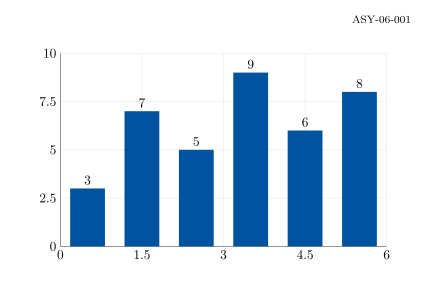
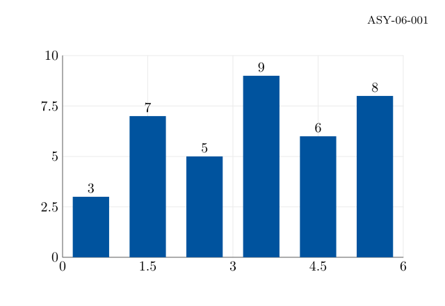
`P(x,y)`	Use the same scale for bars and numeric grid.
`Zero baseline`	Let height encode the actual value.

Complete standalone Asymptote program

settings.tex="pdflatex";
settings.outformat="pdf";
settings.render=0;
settings.prc=false;
settings.v3d=false;
defaultpen(fontsize(10pt));
pen Blue=rgb(0,84/255.0,159/255.0),Teal=rgb(0,177/255.0,183/255.0);
pen Orange=rgb(246/255.0,168/255.0,0),Green=rgb(87/255.0,171/255.0,39/255.0);
pen Grey=gray(.4),Light=gray(.92),Wash=rgb(232/255.0,241/255.0,250/255.0);
string figureID="ASY-06-001";
size(320,220,IgnoreAspect);
fill(box((0,0),(320,220)),white);
// BEGIN DRAWING
real xmin=0,xmax=6,ymin=0,ymax=10;
pair P(real x,real y) {return (45+245*(x-xmin)/(xmax-xmin),35+145*(y-ymin)/(ymax-ymin));}
for(int i=0;i<=4;++i) {
 real x=xmin+i*(xmax-xmin)/4, y=ymin+i*(ymax-ymin)/4;
 draw(P(x,ymin)--P(x,ymax),Light);
 draw(P(xmin,y)--P(xmax,y),Light);
 label(format("$%.3g$",x),P(x,ymin),S);
 label(format("$%.3g$",y),P(xmin,y),W);
}
draw(P(xmin,ymax)--P(xmin,ymin)--P(xmax,ymin),Grey);
real[] v={3,7,5,9,6,8};
for(int i=0;i<v.length;++i) {
 fill(box(P(i+.18,0),P(i+.82,v[i])),Blue);
 label((string)v[i],P(i+.5,v[i]),N);
}
// END DRAWING
label("ASY-06-001",(310,210),SW,fontsize(8pt));
shipout(figureID);

Download: Asymptote source · SVG figure · Vector PDF · PNG preview

ASY-06-002

Fit a line to observed pairs

Least squares estimates the slope and intercept from the observations. The dots show the original synthetic sample.

Back to figure overview

Asymptote drawing

real xmin=0,xmax=9,ymin=0,ymax=9;
pair P(real x,real y) {return (45+245*(x-xmin)/(xmax-xmin),35+145*(y-ymin)/(ymax-ymin));}
for(int i=0;i<=4;++i) {
 real x=xmin+i*(xmax-xmin)/4, y=ymin+i*(ymax-ymin)/4;
 draw(P(x,ymin)--P(x,ymax),Light);
 draw(P(xmin,y)--P(xmax,y),Light);
 label(format("$%.3g$",x),P(x,ymin),S);
 label(format("$%.3g$",y),P(xmin,y),W);
}
draw(P(xmin,ymax)--P(xmin,ymin)--P(xmax,ymin),Grey);
real[] x={1,2,3,4,5,6,7,8};
real[] y={2.1,2.8,4.2,4,5.6,6.8,6.6,8.1};
real sx=0,sy=0,sxx=0,sxy=0; int n=x.length;
for(int i=0;i<n;++i) {
 sx+=x[i]; sy+=y[i]; sxx+=x[i]^2; sxy+=x[i]*y[i];
 dot(P(x[i],y[i]),Orange+5);
}
real slope=(n*sxy-sx*sy)/(n*sxx-sx^2);
real intercept=(sy-slope*sx)/n;
draw(P(0,intercept)--P(9,intercept+9*slope),Blue+1.5);
write("check: slope="+(string)slope);

Actual output

Fit a line to observed pairs — ASY-06-002 · Rendered by Asymptote

Asymptote · exit 0

Native compiler log

Standard output

check: slope=0.838095238095237

Command or parameter	Meaning
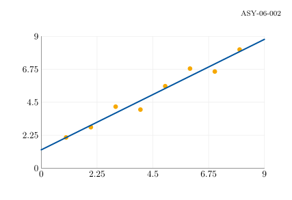
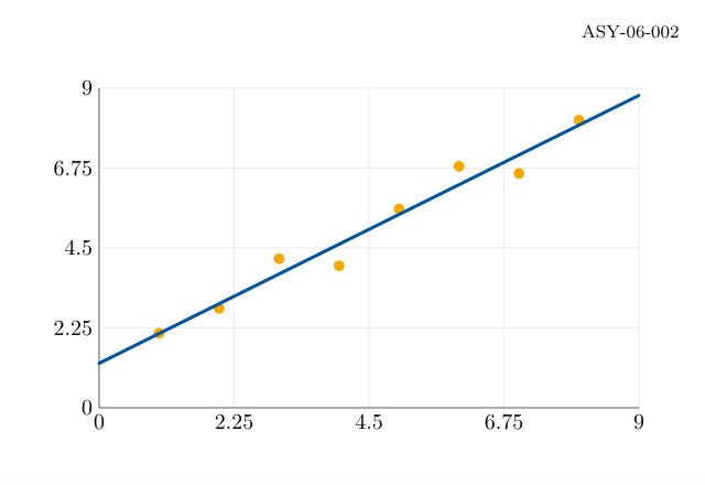
`slope / intercept`	Calculate coefficients from sums over all observations.
`Common axes`	Use identical coordinates for sample points and fitted line.

Complete standalone Asymptote program

settings.tex="pdflatex";
settings.outformat="pdf";
settings.render=0;
settings.prc=false;
settings.v3d=false;
defaultpen(fontsize(10pt));
pen Blue=rgb(0,84/255.0,159/255.0),Teal=rgb(0,177/255.0,183/255.0);
pen Orange=rgb(246/255.0,168/255.0,0),Green=rgb(87/255.0,171/255.0,39/255.0);
pen Grey=gray(.4),Light=gray(.92),Wash=rgb(232/255.0,241/255.0,250/255.0);
string figureID="ASY-06-002";
size(320,220,IgnoreAspect);
fill(box((0,0),(320,220)),white);
// BEGIN DRAWING
real xmin=0,xmax=9,ymin=0,ymax=9;
pair P(real x,real y) {return (45+245*(x-xmin)/(xmax-xmin),35+145*(y-ymin)/(ymax-ymin));}
for(int i=0;i<=4;++i) {
 real x=xmin+i*(xmax-xmin)/4, y=ymin+i*(ymax-ymin)/4;
 draw(P(x,ymin)--P(x,ymax),Light);
 draw(P(xmin,y)--P(xmax,y),Light);
 label(format("$%.3g$",x),P(x,ymin),S);
 label(format("$%.3g$",y),P(xmin,y),W);
}
draw(P(xmin,ymax)--P(xmin,ymin)--P(xmax,ymin),Grey);
real[] x={1,2,3,4,5,6,7,8};
real[] y={2.1,2.8,4.2,4,5.6,6.8,6.6,8.1};
real sx=0,sy=0,sxx=0,sxy=0; int n=x.length;
for(int i=0;i<n;++i) {
 sx+=x[i]; sy+=y[i]; sxx+=x[i]^2; sxy+=x[i]*y[i];
 dot(P(x[i],y[i]),Orange+5);
}
real slope=(n*sxy-sx*sy)/(n*sxx-sx^2);
real intercept=(sy-slope*sx)/n;
draw(P(0,intercept)--P(9,intercept+9*slope),Blue+1.5);
write("check: slope="+(string)slope);
// END DRAWING
label("ASY-06-002",(310,210),SW,fontsize(8pt));
shipout(figureID);

Download: Asymptote source · SVG figure · Vector PDF · PNG preview

ASY-06-003

Bin raw data into a histogram

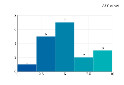
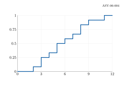
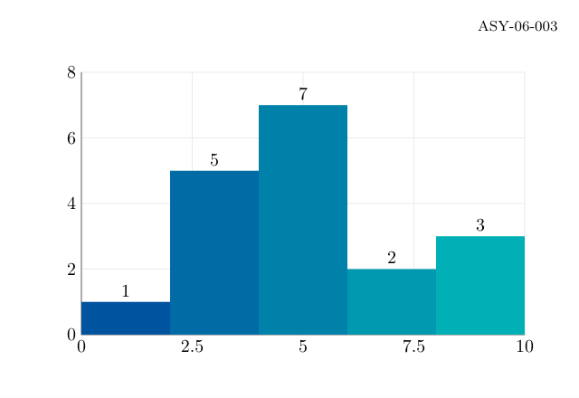
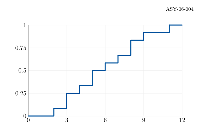
Counts are computed from the observations rather than supplied as bar heights. The bins are left-closed and right-open, with the final endpoint included.

Back to figure overview

Asymptote drawing

real xmin=0,xmax=10,ymin=0,ymax=8;
pair P(real x,real y) {return (45+245*(x-xmin)/(xmax-xmin),35+145*(y-ymin)/(ymax-ymin));}
for(int i=0;i<=4;++i) {
 real x=xmin+i*(xmax-xmin)/4, y=ymin+i*(ymax-ymin)/4;
 draw(P(x,ymin)--P(x,ymax),Light);
 draw(P(xmin,y)--P(xmax,y),Light);
 label(format("$%.3g$",x),P(x,ymin),S);
 label(format("$%.3g$",y),P(xmin,y),W);
}
draw(P(xmin,ymax)--P(xmin,ymin)--P(xmax,ymin),Grey);
real[] v={.8,2.1,2.4,2.8,3.1,3.7,4.1,4.3,4.7,5,5.2,5.5,5.9,6.2,7.4,8.1,8.7,9.2};
int[] count=new int[5];
for(int i=0;i<5;++i) count[i]=0;
for(real value:v) ++count[min(4,(int)floor(value/2))];
int total=0;
for(int i=0;i<5;++i) {
 total+=count[i]; fill(box(P(2*i,0),P(2*i+2,count[i])),interp(Blue,Teal,i/4.0));
 label((string)count[i],P(2*i+1,count[i]),N);
}
write("check: histogram-total="+(string)total);

Actual output

Bin raw data into a histogram — ASY-06-003 · Rendered by Asymptote

Asymptote · exit 0

Native compiler log

Standard output

check: histogram-total=18

Command or parameter	Meaning
`floor(value/2)`	Assign observations to two-unit bins.
`Equal widths`	Use bar height as count for these equal-width bins.

Complete standalone Asymptote program

settings.tex="pdflatex";
settings.outformat="pdf";
settings.render=0;
settings.prc=false;
settings.v3d=false;
defaultpen(fontsize(10pt));
pen Blue=rgb(0,84/255.0,159/255.0),Teal=rgb(0,177/255.0,183/255.0);
pen Orange=rgb(246/255.0,168/255.0,0),Green=rgb(87/255.0,171/255.0,39/255.0);
pen Grey=gray(.4),Light=gray(.92),Wash=rgb(232/255.0,241/255.0,250/255.0);
string figureID="ASY-06-003";
size(320,220,IgnoreAspect);
fill(box((0,0),(320,220)),white);
// BEGIN DRAWING
real xmin=0,xmax=10,ymin=0,ymax=8;
pair P(real x,real y) {return (45+245*(x-xmin)/(xmax-xmin),35+145*(y-ymin)/(ymax-ymin));}
for(int i=0;i<=4;++i) {
 real x=xmin+i*(xmax-xmin)/4, y=ymin+i*(ymax-ymin)/4;
 draw(P(x,ymin)--P(x,ymax),Light);
 draw(P(xmin,y)--P(xmax,y),Light);
 label(format("$%.3g$",x),P(x,ymin),S);
 label(format("$%.3g$",y),P(xmin,y),W);
}
draw(P(xmin,ymax)--P(xmin,ymin)--P(xmax,ymin),Grey);
real[] v={.8,2.1,2.4,2.8,3.1,3.7,4.1,4.3,4.7,5,5.2,5.5,5.9,6.2,7.4,8.1,8.7,9.2};
int[] count=new int[5];
for(int i=0;i<5;++i) count[i]=0;
for(real value:v) ++count[min(4,(int)floor(value/2))];
int total=0;
for(int i=0;i<5;++i) {
 total+=count[i]; fill(box(P(2*i,0),P(2*i+2,count[i])),interp(Blue,Teal,i/4.0));
 label((string)count[i],P(2*i+1,count[i]),N);
}
write("check: histogram-total="+(string)total);
// END DRAWING
label("ASY-06-003",(310,210),SW,fontsize(8pt));
shipout(figureID);

Download: Asymptote source · SVG figure · Vector PDF · PNG preview

ASY-06-004

Calculate an empirical distribution

Sort the sample, group equal observations and advance by their combined probability. The step function is right-continuous.

Back to figure overview

Asymptote drawing

real xmin=0,xmax=12,ymin=0,ymax=1;
pair P(real x,real y) {return (45+245*(x-xmin)/(xmax-xmin),35+145*(y-ymin)/(ymax-ymin));}
for(int i=0;i<=4;++i) {
 real x=xmin+i*(xmax-xmin)/4, y=ymin+i*(ymax-ymin)/4;
 draw(P(x,ymin)--P(x,ymax),Light);
 draw(P(xmin,y)--P(xmax,y),Light);
 label(format("$%.3g$",x),P(x,ymin),S);
 label(format("$%.3g$",y),P(xmin,y),W);
}
draw(P(xmin,ymax)--P(xmin,ymin)--P(xmax,ymin),Grey);
real[] v=sort(new real[] {2,3,3,4,5,5,6,7,8,8,9,11});
int n=v.length,i=0; pair last=P(0,0);
while(i<n) {
 int j=i+1; while(j<n && v[j]==v[i]) ++j;
 pair before=P(v[i],i/(real)n),after=P(v[i],j/(real)n);
 draw(last--before--after,Blue+1.6); last=after; i=j;
}
draw(last--P(12,1),Blue+1.6);
write("check: ecdf-final="+(string)(i/(real)n));

Actual output

Calculate an empirical distribution — ASY-06-004 · Rendered by Asymptote

Asymptote · exit 0

Native compiler log

Standard output

check: ecdf-final=1

Command or parameter	Meaning
`sort`	Create an ordered copy of the observations.
`Grouped ties`	Move vertically by their total mass.
`Right-continuous`	The value at each observation includes that observation.

Complete standalone Asymptote program

settings.tex="pdflatex";
settings.outformat="pdf";
settings.render=0;
settings.prc=false;
settings.v3d=false;
defaultpen(fontsize(10pt));
pen Blue=rgb(0,84/255.0,159/255.0),Teal=rgb(0,177/255.0,183/255.0);
pen Orange=rgb(246/255.0,168/255.0,0),Green=rgb(87/255.0,171/255.0,39/255.0);
pen Grey=gray(.4),Light=gray(.92),Wash=rgb(232/255.0,241/255.0,250/255.0);
string figureID="ASY-06-004";
size(320,220,IgnoreAspect);
fill(box((0,0),(320,220)),white);
// BEGIN DRAWING
real xmin=0,xmax=12,ymin=0,ymax=1;
pair P(real x,real y) {return (45+245*(x-xmin)/(xmax-xmin),35+145*(y-ymin)/(ymax-ymin));}
for(int i=0;i<=4;++i) {
 real x=xmin+i*(xmax-xmin)/4, y=ymin+i*(ymax-ymin)/4;
 draw(P(x,ymin)--P(x,ymax),Light);
 draw(P(xmin,y)--P(xmax,y),Light);
 label(format("$%.3g$",x),P(x,ymin),S);
 label(format("$%.3g$",y),P(xmin,y),W);
}
draw(P(xmin,ymax)--P(xmin,ymin)--P(xmax,ymin),Grey);
real[] v=sort(new real[] {2,3,3,4,5,5,6,7,8,8,9,11});
int n=v.length,i=0; pair last=P(0,0);
while(i<n) {
 int j=i+1; while(j<n && v[j]==v[i]) ++j;
 pair before=P(v[i],i/(real)n),after=P(v[i],j/(real)n);
 draw(last--before--after,Blue+1.6); last=after; i=j;
}
draw(last--P(12,1),Blue+1.6);
write("check: ecdf-final="+(string)(i/(real)n));
// END DRAWING
label("ASY-06-004",(310,210),SW,fontsize(8pt));
shipout(figureID);

Download: Asymptote source · SVG figure · Vector PDF · PNG preview

ASY-06-005

Construct a box plot from observations

The median and quartiles are calculated after sorting. Whiskers explicitly show the minimum and maximum; they do not apply an outlier rule.

Back to figure overview

Asymptote drawing

real[] v=sort(new real[] {2,3,3,4,4,5,6,7,8,8,9,11});
real q1=(v[2]+v[3])/2,median=(v[5]+v[6])/2,q3=(v[8]+v[9])/2;
real X(real x) {return 40+20*x;}
draw((X(v[0]),105)--(X(v[11]),105),Blue);
filldraw(box((X(q1),80),(X(q3),130)),Wash,Blue);
draw((X(median),80)--(X(median),130),Orange+2);
for(int i:new int[] {0,11}) draw((X(v[i]),90)--(X(v[i]),120),Blue);
for(int i=0;i<v.length;++i) dot((X(v[i]),165+4*(i%2)),Teal+3);
draw((40,45)--(280,45),Grey);
for(int x=0;x<=12;x+=3) label((string)x,(X(x),45),S);
write("check: quartiles="+(string)q1+","+(string)median+","+(string)q3);

Actual output

Construct a box plot from observations — ASY-06-005 · Rendered by Asymptote

Asymptote · exit 0

Native compiler log

Standard output

check: quartiles=3.5,5.5,8

Command or parameter	Meaning
`Median of halves`	Use 3.5, 5.5 and 8 for this sample.
`Whiskers`	Use the sample minimum 2 and maximum 11.
`Raw dots`	Expose the underlying observations.

Complete standalone Asymptote program

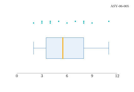
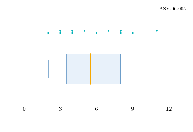
settings.tex="pdflatex";
settings.outformat="pdf";
settings.render=0;
settings.prc=false;
settings.v3d=false;
defaultpen(fontsize(10pt));
pen Blue=rgb(0,84/255.0,159/255.0),Teal=rgb(0,177/255.0,183/255.0);
pen Orange=rgb(246/255.0,168/255.0,0),Green=rgb(87/255.0,171/255.0,39/255.0);
pen Grey=gray(.4),Light=gray(.92),Wash=rgb(232/255.0,241/255.0,250/255.0);
string figureID="ASY-06-005";
size(320,220,IgnoreAspect);
fill(box((0,0),(320,220)),white);
// BEGIN DRAWING
real[] v=sort(new real[] {2,3,3,4,4,5,6,7,8,8,9,11});
real q1=(v[2]+v[3])/2,median=(v[5]+v[6])/2,q3=(v[8]+v[9])/2;
real X(real x) {return 40+20*x;}
draw((X(v[0]),105)--(X(v[11]),105),Blue);
filldraw(box((X(q1),80),(X(q3),130)),Wash,Blue);
draw((X(median),80)--(X(median),130),Orange+2);
for(int i:new int[] {0,11}) draw((X(v[i]),90)--(X(v[i]),120),Blue);
for(int i=0;i<v.length;++i) dot((X(v[i]),165+4*(i%2)),Teal+3);
draw((40,45)--(280,45),Grey);
for(int x=0;x<=12;x+=3) label((string)x,(X(x),45),S);
write("check: quartiles="+(string)q1+","+(string)median+","+(string)q3);
// END DRAWING
label("ASY-06-005",(310,210),SW,fontsize(8pt));
shipout(figureID);

Download: Asymptote source · SVG figure · Vector PDF · PNG preview

ASY-06-006

Estimate a violin density

Gaussian kernels are centred on the sample values. The width represents a density estimate; the dots show the same raw observations.

Back to figure overview

Asymptote drawing

import graph;
real[] v={2,2.4,3,3.2,3.4,5.7,6,6.4,7,7.5};
real h=.45;
real density(real y) {
 real s=0; for(real value:v) s+=exp(-.5*((y-value)/h)^2);
 return s/(v.length*h*sqrt(2*pi));
}
pair left(real y) {return (160-110*density(y),30+18*y);}
pair right(real y) {return (160+110*density(y),30+18*y);}
path a=graph(left,0,9,200),b=graph(right,0,9,200);
filldraw(a--reverse(b)--cycle,Wash,Blue);
for(int i=0;i<v.length;++i) dot((160+4*((i%3)-1),30+18*v[i]),Orange+4);
for(int y=0;y<=8;y+=2) label((string)y,(85,30+18*y),W);
label("KDE bandwidth 0.45",(160,15));

Actual output

Estimate a violin density — ASY-06-006 · Rendered by Asymptote

Asymptote · exit 0

Native compiler log

Compilation completed successfully. No compiler messages were emitted.

Command or parameter	Meaning
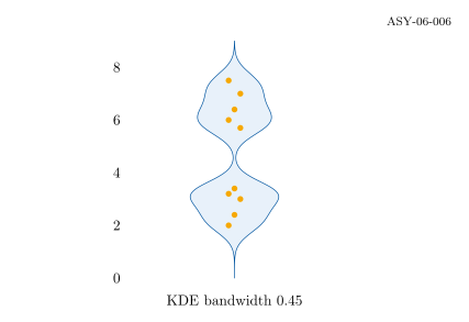
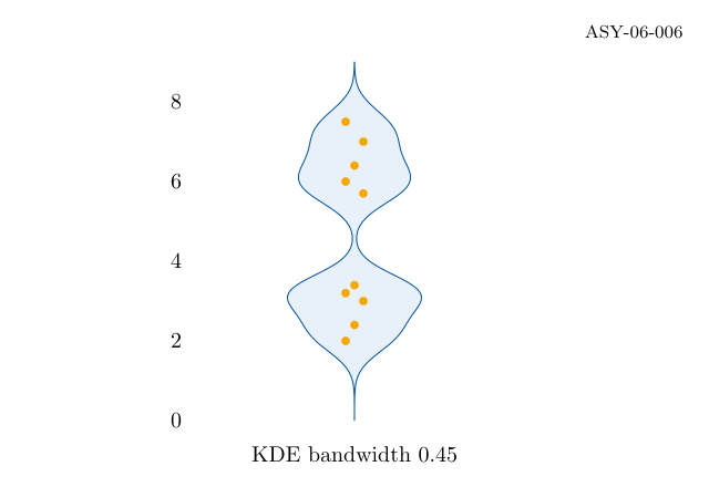
`h=.45`	Use one bandwidth in the data units.
`Gaussian kernel`	Sum normal-shaped contributions at observed values.
`Mirrored density`	Trace one side up and the other down.

Complete standalone Asymptote program

settings.tex="pdflatex";
settings.outformat="pdf";
settings.render=0;
settings.prc=false;
settings.v3d=false;
defaultpen(fontsize(10pt));
pen Blue=rgb(0,84/255.0,159/255.0),Teal=rgb(0,177/255.0,183/255.0);
pen Orange=rgb(246/255.0,168/255.0,0),Green=rgb(87/255.0,171/255.0,39/255.0);
pen Grey=gray(.4),Light=gray(.92),Wash=rgb(232/255.0,241/255.0,250/255.0);
string figureID="ASY-06-006";
size(320,220,IgnoreAspect);
fill(box((0,0),(320,220)),white);
// BEGIN DRAWING
import graph;
real[] v={2,2.4,3,3.2,3.4,5.7,6,6.4,7,7.5};
real h=.45;
real density(real y) {
 real s=0; for(real value:v) s+=exp(-.5*((y-value)/h)^2);
 return s/(v.length*h*sqrt(2*pi));
}
pair left(real y) {return (160-110*density(y),30+18*y);}
pair right(real y) {return (160+110*density(y),30+18*y);}
path a=graph(left,0,9,200),b=graph(right,0,9,200);
filldraw(a--reverse(b)--cycle,Wash,Blue);
for(int i=0;i<v.length;++i) dot((160+4*((i%3)-1),30+18*v[i]),Orange+4);
for(int y=0;y<=8;y+=2) label((string)y,(85,30+18*y),W);
label("KDE bandwidth 0.45",(160,15));
// END DRAWING
label("ASY-06-006",(310,210),SW,fontsize(8pt));
shipout(figureID);

Download: Asymptote source · SVG figure · Vector PDF · PNG preview

07 · Scalar and vector fields

ASY-07-001

Draw quadratic level sets

The contour module computes level lines from a scalar function. Elliptical contours reveal different rates of change along the two axes.

Back to figure overview

Asymptote drawing

import graph;
import contour;
real f(real x,real y) {return x*x+2*y*y;}
draw(contour(f,(-2,-1.5),(2,1.5),new real[] {.3,.8,1.5,2.5,3.5},60),Blue+1.2);
xaxis("$x$",BottomTop,Ticks); yaxis("$y$",LeftRight,Ticks);

Actual output

Draw quadratic level sets — ASY-07-001 · Rendered by Asymptote

Asymptote · exit 0

Native compiler log

Compilation completed successfully. No compiler messages were emitted.

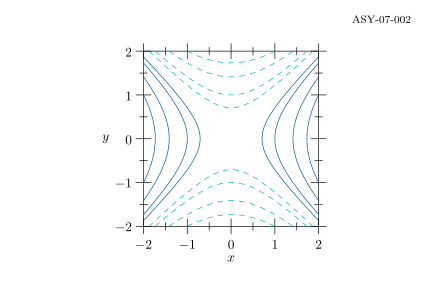
Command or parameter	Meaning
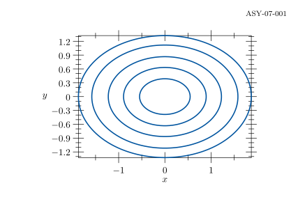
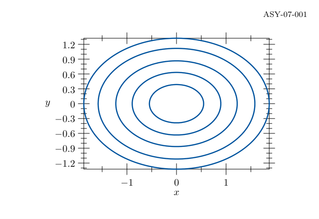
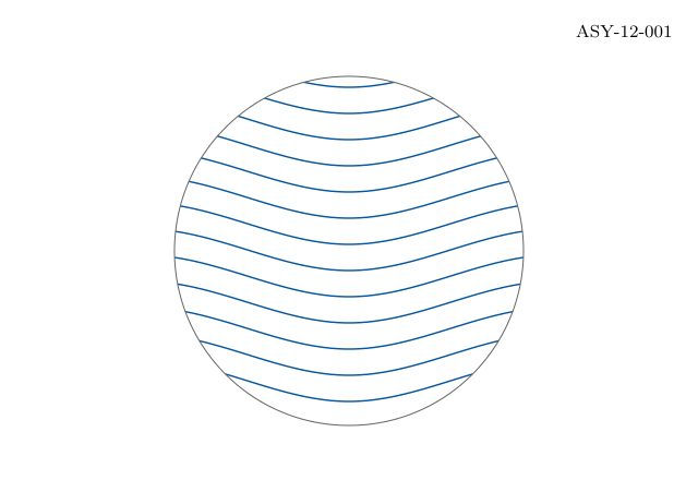
`contour(f,a,b,levels,n)`	Compute level lines on a sampled rectangular domain.
`Levels`	Use explicit scalar values, not nested ellipse radii.

Complete standalone Asymptote program

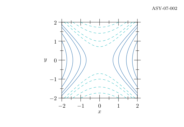
settings.tex="pdflatex";
settings.outformat="pdf";
settings.render=0;
settings.prc=false;
settings.v3d=false;
defaultpen(fontsize(10pt));
pen Blue=rgb(0,84/255.0,159/255.0),Teal=rgb(0,177/255.0,183/255.0);
pen Orange=rgb(246/255.0,168/255.0,0),Green=rgb(87/255.0,171/255.0,39/255.0);
pen Grey=gray(.4),Light=gray(.92),Wash=rgb(232/255.0,241/255.0,250/255.0);
string figureID="ASY-07-001";
size(270,165);
// BEGIN DRAWING
import graph;
import contour;
real f(real x,real y) {return x*x+2*y*y;}
draw(contour(f,(-2,-1.5),(2,1.5),new real[] {.3,.8,1.5,2.5,3.5},60),Blue+1.2);
xaxis("$x$",BottomTop,Ticks); yaxis("$y$",LeftRight,Ticks);
// END DRAWING
picture drawing=currentpicture;
currentpicture=new picture;
size(320,220,IgnoreAspect);
fill(box((0,0),(320,220)),white);
add(drawing.fit(),(160,105),align=0);
label("ASY-07-001",(310,210),SW,fontsize(8pt));
shipout(figureID);

Download: Asymptote source · SVG figure · Vector PDF · PNG preview

ASY-07-002

Distinguish positive and negative contours

A saddle field has positive and negative branches. Line style communicates sign without relying on colour alone.

Back to figure overview

Compare with ASY-07-001 · Draw quadratic level sets.

Asymptote drawing

import graph;
import contour;
real f(real x,real y) {return x*x-y*y;}
draw(contour(f,(-2,-2),(2,2),new real[] {.5,1,2,3},60),Blue);
draw(contour(f,(-2,-2),(2,2),new real[] {-.5,-1,-2,-3},60),Teal+dashed);
xaxis("$x$",BottomTop,Ticks); yaxis("$y$",LeftRight,Ticks);

Actual output

Distinguish positive and negative contours — ASY-07-002 · Rendered by Asymptote

Asymptote · exit 0

Native compiler log

Compilation completed successfully. No compiler messages were emitted.

Command or parameter	Meaning
`Two level arrays`	Group contours by sign.
`dashed`	Provide a second visual channel for negative values.

Complete standalone Asymptote program

settings.tex="pdflatex";
settings.outformat="pdf";
settings.render=0;
settings.prc=false;
settings.v3d=false;
defaultpen(fontsize(10pt));
pen Blue=rgb(0,84/255.0,159/255.0),Teal=rgb(0,177/255.0,183/255.0);
pen Orange=rgb(246/255.0,168/255.0,0),Green=rgb(87/255.0,171/255.0,39/255.0);
pen Grey=gray(.4),Light=gray(.92),Wash=rgb(232/255.0,241/255.0,250/255.0);
string figureID="ASY-07-002";
size(270,165);
// BEGIN DRAWING
import graph;
import contour;
real f(real x,real y) {return x*x-y*y;}
draw(contour(f,(-2,-2),(2,2),new real[] {.5,1,2,3},60),Blue);
draw(contour(f,(-2,-2),(2,2),new real[] {-.5,-1,-2,-3},60),Teal+dashed);
xaxis("$x$",BottomTop,Ticks); yaxis("$y$",LeftRight,Ticks);
// END DRAWING
picture drawing=currentpicture;
currentpicture=new picture;
size(320,220,IgnoreAspect);
fill(box((0,0),(320,220)),white);
add(drawing.fit(),(160,105),align=0);
label("ASY-07-002",(310,210),SW,fontsize(8pt));
shipout(figureID);

Download: Asymptote source · SVG figure · Vector PDF · PNG preview

ASY-07-003

Colour a triangulated field

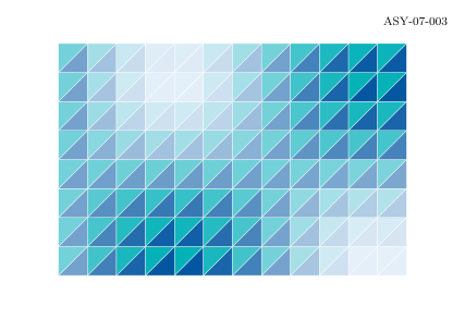
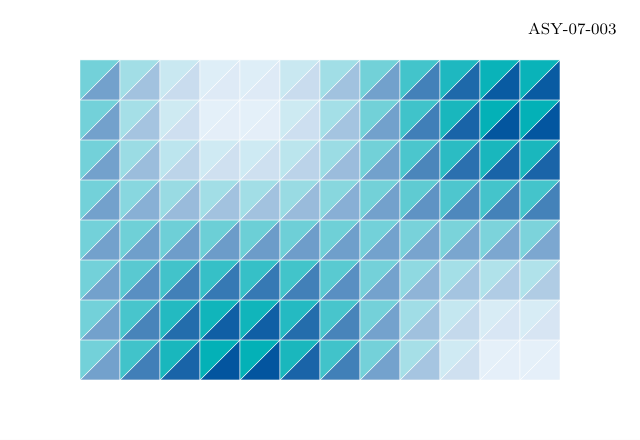
A scalar calculation assigns one colour to each triangular cell. This is a discrete field illustration, with a visible mesh rather than a raster interpolation.

Back to figure overview

Asymptote drawing

for(int i=0;i<12;++i) for(int j=0;j<8;++j) {
 pair a=(40+20*i,30+20*j),b=a+(20,0),c=a+(20,20),d=a+(0,20);
 real t=(1+sin(.45*i)*cos(.5*j))/2;
 filldraw(a--b--c--cycle,interp(Wash,Blue,t),white+.25);
 filldraw(a--c--d--cycle,interp(Wash,Teal,t),white+.25);
}

Actual output

Colour a triangulated field — ASY-07-003 · Rendered by Asymptote

Asymptote · exit 0

Native compiler log

Compilation completed successfully. No compiler messages were emitted.

Command or parameter	Meaning
`Cell value`	Evaluate the field once per rectangular cell.
`Two triangles`	Split each rectangle along its diagonal.
`Flat colour`	Each triangular cell has one fill value.

Complete standalone Asymptote program

settings.tex="pdflatex";
settings.outformat="pdf";
settings.render=0;
settings.prc=false;
settings.v3d=false;
defaultpen(fontsize(10pt));
pen Blue=rgb(0,84/255.0,159/255.0),Teal=rgb(0,177/255.0,183/255.0);
pen Orange=rgb(246/255.0,168/255.0,0),Green=rgb(87/255.0,171/255.0,39/255.0);
pen Grey=gray(.4),Light=gray(.92),Wash=rgb(232/255.0,241/255.0,250/255.0);
string figureID="ASY-07-003";
size(320,220,IgnoreAspect);
fill(box((0,0),(320,220)),white);
// BEGIN DRAWING
for(int i=0;i<12;++i) for(int j=0;j<8;++j) {
 pair a=(40+20*i,30+20*j),b=a+(20,0),c=a+(20,20),d=a+(0,20);
 real t=(1+sin(.45*i)*cos(.5*j))/2;
 filldraw(a--b--c--cycle,interp(Wash,Blue,t),white+.25);
 filldraw(a--c--d--cycle,interp(Wash,Teal,t),white+.25);
}
// END DRAWING
label("ASY-07-003",(310,210),SW,fontsize(8pt));
shipout(figureID);

Download: Asymptote source · SVG figure · Vector PDF · PNG preview

ASY-07-004

Normalize a rotational vector field

Equal-length arrows reveal direction. Their magnitude has deliberately been removed by normalization, and the zero vector is skipped.

Back to figure overview

Asymptote drawing

for(int i=-4;i<=4;++i) for(int j=-2;j<=2;++j) {
 pair v=(-j,i),p=(160+27*i,105+30*j);
 if(abs(v)>0) draw(p-6*unit(v)--p+6*unit(v),Blue,Arrow(3));
}

Actual output

Normalize a rotational vector field — ASY-07-004 · Rendered by Asymptote

Asymptote · exit 0

Native compiler log

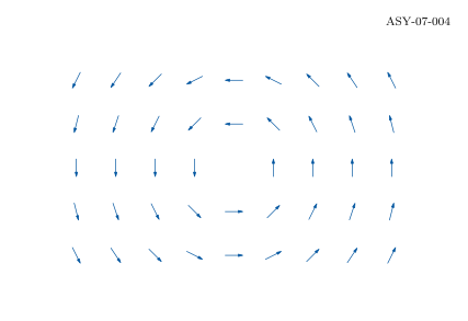
Compilation completed successfully. No compiler messages were emitted.

Command or parameter	Meaning
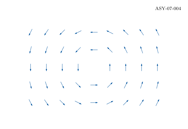
`F(x,y)=(-y,x)`	A rotational vector field.
`unit(v)`	Keep direction while normalizing length.
`Zero vector`	Skip normalization at the origin.

Complete standalone Asymptote program

settings.tex="pdflatex";
settings.outformat="pdf";
settings.render=0;
settings.prc=false;
settings.v3d=false;
defaultpen(fontsize(10pt));
pen Blue=rgb(0,84/255.0,159/255.0),Teal=rgb(0,177/255.0,183/255.0);
pen Orange=rgb(246/255.0,168/255.0,0),Green=rgb(87/255.0,171/255.0,39/255.0);
pen Grey=gray(.4),Light=gray(.92),Wash=rgb(232/255.0,241/255.0,250/255.0);
string figureID="ASY-07-004";
size(320,220,IgnoreAspect);
fill(box((0,0),(320,220)),white);
// BEGIN DRAWING
for(int i=-4;i<=4;++i) for(int j=-2;j<=2;++j) {
 pair v=(-j,i),p=(160+27*i,105+30*j);
 if(abs(v)>0) draw(p-6*unit(v)--p+6*unit(v),Blue,Arrow(3));
}
// END DRAWING
label("ASY-07-004",(310,210),SW,fontsize(8pt));
shipout(figureID);

Download: Asymptote source · SVG figure · Vector PDF · PNG preview

ASY-07-005

Preserve vector magnitudes

Each arrow now uses one common conversion factor. Length shows field magnitude as well as direction.

Back to figure overview

Compare with ASY-07-004 · Normalize a rotational vector field.

Asymptote drawing

for(int i=-4;i<=4;++i) for(int j=-2;j<=2;++j) {
 pair v=5*(-j,i),p=(160+27*i,105+30*j);
 if(abs(v)>0) draw(p-.5*v--p+.5*v,Blue,Arrow(3));
}

Actual output

Preserve vector magnitudes — ASY-07-005 · Rendered by Asymptote

Asymptote · exit 0

Native compiler log

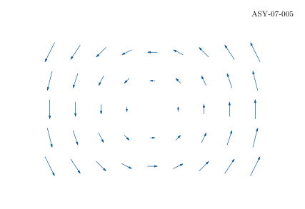
Compilation completed successfully. No compiler messages were emitted.

Command or parameter	Meaning
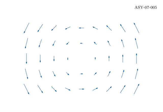
`Common scale`	Five drawing units represent one field unit.
`Centred arrows`	Keep the sample location at each arrow midpoint.

Complete standalone Asymptote program

settings.tex="pdflatex";
settings.outformat="pdf";
settings.render=0;
settings.prc=false;
settings.v3d=false;
defaultpen(fontsize(10pt));
pen Blue=rgb(0,84/255.0,159/255.0),Teal=rgb(0,177/255.0,183/255.0);
pen Orange=rgb(246/255.0,168/255.0,0),Green=rgb(87/255.0,171/255.0,39/255.0);
pen Grey=gray(.4),Light=gray(.92),Wash=rgb(232/255.0,241/255.0,250/255.0);
string figureID="ASY-07-005";
size(320,220,IgnoreAspect);
fill(box((0,0),(320,220)),white);
// BEGIN DRAWING
for(int i=-4;i<=4;++i) for(int j=-2;j<=2;++j) {
 pair v=5*(-j,i),p=(160+27*i,105+30*j);
 if(abs(v)>0) draw(p-.5*v--p+.5*v,Blue,Arrow(3));
}
// END DRAWING
label("ASY-07-005",(310,210),SW,fontsize(8pt));
shipout(figureID);

Download: Asymptote source · SVG figure · Vector PDF · PNG preview

ASY-07-006

Integrate approximate streamlines

Explicit Euler steps follow the vector field. A small fixed step makes the numerical approximation visible and reproducible.

Back to figure overview

Asymptote drawing

for(int k=1;k<=5;++k) {
 pair q=(.18*k,0); guide trajectory=q;
 real h=.012;
 for(int i=0;i<520;++i) {
  q+=h*(-q.y,q.x); trajectory=trajectory--q;
 }
 draw(shift(160,105)*xscale(100)*yscale(75)*trajectory,
      interp(Blue,Teal,k/5.0));
}

Actual output

Integrate approximate streamlines — ASY-07-006 · Rendered by Asymptote

Asymptote · exit 0

Native compiler log

Compilation completed successfully. No compiler messages were emitted.

Command or parameter	Meaning
`Euler update`	Advance position using the current field value.
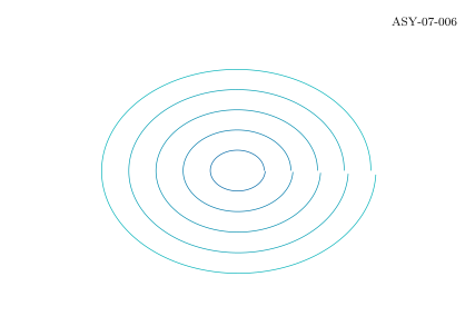
`Approximation`	Euler introduces a small outward drift; it is not an exact circle.
`h=.012`	Set the integration step, independently of stroke width.

Complete standalone Asymptote program

settings.tex="pdflatex";
settings.outformat="pdf";
settings.render=0;
settings.prc=false;
settings.v3d=false;
defaultpen(fontsize(10pt));
pen Blue=rgb(0,84/255.0,159/255.0),Teal=rgb(0,177/255.0,183/255.0);
pen Orange=rgb(246/255.0,168/255.0,0),Green=rgb(87/255.0,171/255.0,39/255.0);
pen Grey=gray(.4),Light=gray(.92),Wash=rgb(232/255.0,241/255.0,250/255.0);
string figureID="ASY-07-006";
size(320,220,IgnoreAspect);
fill(box((0,0),(320,220)),white);
// BEGIN DRAWING
for(int k=1;k<=5;++k) {
 pair q=(.18*k,0); guide trajectory=q;
 real h=.012;
 for(int i=0;i<520;++i) {
  q+=h*(-q.y,q.x); trajectory=trajectory--q;
 }
 draw(shift(160,105)*xscale(100)*yscale(75)*trajectory,
      interp(Blue,Teal,k/5.0));
}
// END DRAWING
label("ASY-07-006",(310,210),SW,fontsize(8pt));
shipout(figureID);

Download: Asymptote source · SVG figure · Vector PDF · PNG preview

08 · Patterns and complex maps

ASY-08-001

Subdivide a triangle recursively

A bounded recursion leaves three smaller corner triangles at each level. The base case produces the final filled pieces.

Back to figure overview

Asymptote drawing

void subdivide(pair a,pair b,pair c,int depth) {
 if(depth==0) fill(a--b--c--cycle,Blue);
 else {
  subdivide(a,(a+b)/2,(a+c)/2,depth-1);
  subdivide((a+b)/2,b,(b+c)/2,depth-1);
  subdivide((a+c)/2,(b+c)/2,c,depth-1);
 }
}
subdivide((45,35),(275,35),(160,190),5);

Actual output

Subdivide a triangle recursively — ASY-08-001 · Rendered by Asymptote

Asymptote · exit 0

Native compiler log

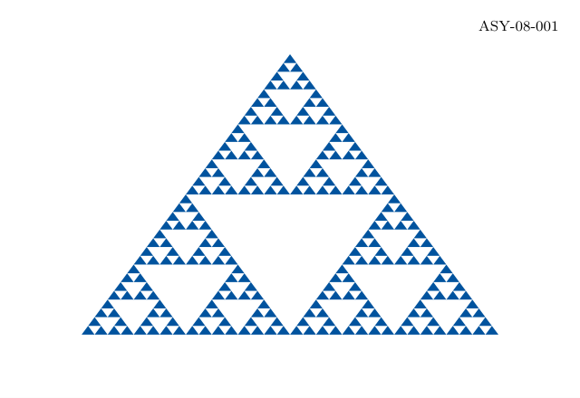
Compilation completed successfully. No compiler messages were emitted.

Command or parameter	Meaning
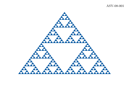
`depth==0`	Define an explicit termination condition.
`Midpoints`	Reuse affine interpolation at every level.

Complete standalone Asymptote program

settings.tex="pdflatex";
settings.outformat="pdf";
settings.render=0;
settings.prc=false;
settings.v3d=false;
defaultpen(fontsize(10pt));
pen Blue=rgb(0,84/255.0,159/255.0),Teal=rgb(0,177/255.0,183/255.0);
pen Orange=rgb(246/255.0,168/255.0,0),Green=rgb(87/255.0,171/255.0,39/255.0);
pen Grey=gray(.4),Light=gray(.92),Wash=rgb(232/255.0,241/255.0,250/255.0);
string figureID="ASY-08-001";
size(320,220,IgnoreAspect);
fill(box((0,0),(320,220)),white);
// BEGIN DRAWING
void subdivide(pair a,pair b,pair c,int depth) {
 if(depth==0) fill(a--b--c--cycle,Blue);
 else {
  subdivide(a,(a+b)/2,(a+c)/2,depth-1);
  subdivide((a+b)/2,b,(b+c)/2,depth-1);
  subdivide((a+c)/2,(b+c)/2,c,depth-1);
 }
}
subdivide((45,35),(275,35),(160,190),5);
// END DRAWING
label("ASY-08-001",(310,210),SW,fontsize(8pt));
shipout(figureID);

Download: Asymptote source · SVG figure · Vector PDF · PNG preview

ASY-08-002

Build a rosette from one petal

Rotation repeats a single curved path. Colour changes follow the same loop index, keeping geometry and styling easy to vary independently.

Back to figure overview

Asymptote drawing

path petal=(0,0)..(35,25)..(70,0)..(35,-25)..cycle;
for(int k=0;k<18;++k)
 draw(shift(160,105)*rotate(20*k)*petal,interp(Blue,Teal,k/17.0));

Actual output

Build a rosette from one petal — ASY-08-002 · Rendered by Asymptote

Asymptote · exit 0

Native compiler log

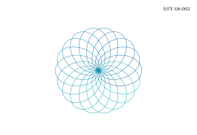
Compilation completed successfully. No compiler messages were emitted.

Command or parameter	Meaning
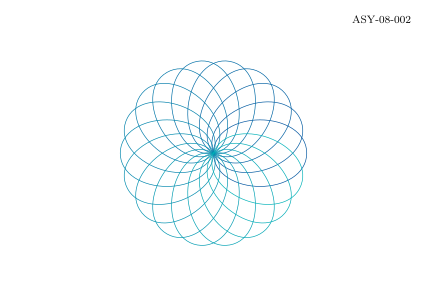
`One motif`	Define the path once.
`rotate(20*k)`	Distribute eighteen copies around a full turn.

Complete standalone Asymptote program

settings.tex="pdflatex";
settings.outformat="pdf";
settings.render=0;
settings.prc=false;
settings.v3d=false;
defaultpen(fontsize(10pt));
pen Blue=rgb(0,84/255.0,159/255.0),Teal=rgb(0,177/255.0,183/255.0);
pen Orange=rgb(246/255.0,168/255.0,0),Green=rgb(87/255.0,171/255.0,39/255.0);
pen Grey=gray(.4),Light=gray(.92),Wash=rgb(232/255.0,241/255.0,250/255.0);
string figureID="ASY-08-002";
size(320,220,IgnoreAspect);
fill(box((0,0),(320,220)),white);
// BEGIN DRAWING
path petal=(0,0)..(35,25)..(70,0)..(35,-25)..cycle;
for(int k=0;k<18;++k)
 draw(shift(160,105)*rotate(20*k)*petal,interp(Blue,Teal,k/17.0));
// END DRAWING
label("ASY-08-002",(310,210),SW,fontsize(8pt));
shipout(figureID);

Download: Asymptote source · SVG figure · Vector PDF · PNG preview

ASY-08-003

Reveal a moire pattern

Two regular ring families interfere visually. The apparent texture comes entirely from vector strokes.

Back to figure overview

Asymptote drawing

for(int k=1;k<=18;++k) {
 draw(circle((140,105),4.5*k),Blue+.35);
 draw(circle((180,105),4.5*k),Teal+.35);
}

Actual output

Reveal a moire pattern — ASY-08-003 · Rendered by Asymptote

Asymptote · exit 0

Native compiler log

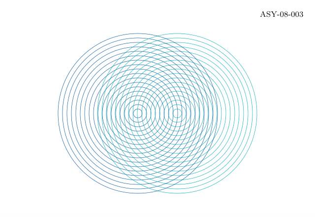
Compilation completed successfully. No compiler messages were emitted.

Command or parameter	Meaning
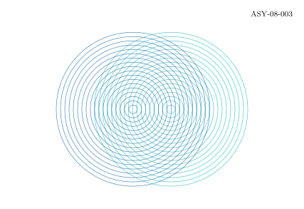
`Two centres`	Offset identical families by forty units.
`Constant spacing`	Keep the pattern regular before the families overlap.

Complete standalone Asymptote program

settings.tex="pdflatex";
settings.outformat="pdf";
settings.render=0;
settings.prc=false;
settings.v3d=false;
defaultpen(fontsize(10pt));
pen Blue=rgb(0,84/255.0,159/255.0),Teal=rgb(0,177/255.0,183/255.0);
pen Orange=rgb(246/255.0,168/255.0,0),Green=rgb(87/255.0,171/255.0,39/255.0);
pen Grey=gray(.4),Light=gray(.92),Wash=rgb(232/255.0,241/255.0,250/255.0);
string figureID="ASY-08-003";
size(320,220,IgnoreAspect);
fill(box((0,0),(320,220)),white);
// BEGIN DRAWING
for(int k=1;k<=18;++k) {
 draw(circle((140,105),4.5*k),Blue+.35);
 draw(circle((180,105),4.5*k),Teal+.35);
}
// END DRAWING
label("ASY-08-003",(310,210),SW,fontsize(8pt));
shipout(figureID);

Download: Asymptote source · SVG figure · Vector PDF · PNG preview

ASY-08-004

Draw a logarithmic spiral

Radius grows exponentially as angle increases linearly. The dots are separated by equal angular steps, not equal arc lengths.

Back to figure overview

Asymptote drawing

import graph;
pair spiral(real t) {return (155,105)+2*exp(.16*t)*dir(degrees(t));}
draw(graph(spiral,0,7*pi,600),Blue+1.5);
for(int k=0;k<=14;++k) dot(spiral(k*pi/2),Teal+3);

Actual output

Draw a logarithmic spiral — ASY-08-004 · Rendered by Asymptote

Asymptote · exit 0

Native compiler log

Compilation completed successfully. No compiler messages were emitted.

Command or parameter	Meaning
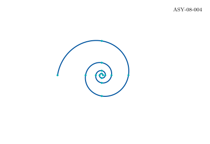
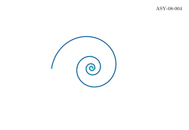
`exp(.16*t)`	Set the radial growth rate.
`degrees(t)`	Convert radians to the degree argument of dir.

Complete standalone Asymptote program

settings.tex="pdflatex";
settings.outformat="pdf";
settings.render=0;
settings.prc=false;
settings.v3d=false;
defaultpen(fontsize(10pt));
pen Blue=rgb(0,84/255.0,159/255.0),Teal=rgb(0,177/255.0,183/255.0);
pen Orange=rgb(246/255.0,168/255.0,0),Green=rgb(87/255.0,171/255.0,39/255.0);
pen Grey=gray(.4),Light=gray(.92),Wash=rgb(232/255.0,241/255.0,250/255.0);
string figureID="ASY-08-004";
size(320,220,IgnoreAspect);
fill(box((0,0),(320,220)),white);
// BEGIN DRAWING
import graph;
pair spiral(real t) {return (155,105)+2*exp(.16*t)*dir(degrees(t));}
draw(graph(spiral,0,7*pi,600),Blue+1.5);
for(int k=0;k<=14;++k) dot(spiral(k*pi/2),Teal+3);
// END DRAWING
label("ASY-08-004",(310,210),SW,fontsize(8pt));
shipout(figureID);

Download: Asymptote source · SVG figure · Vector PDF · PNG preview

ASY-08-005

Compare phase-shifted trajectories

A small-multiple layout reveals how one phase parameter changes a Lissajous curve. Frequencies and panel scale stay fixed.

Back to figure overview

Asymptote drawing

import graph;
for(int j=0;j<2;++j) for(int i=0;i<3;++i) {
 real phase=(i+3*j)*pi/6;
 pair f(real t) {return (65+95*i,65+85*j)+(35*sin(2*t+phase),30*cos(3*t));}
 draw(graph(f,0,2*pi,240),interp(Blue,Teal,(i+3*j)/5.0));
}

Actual output

Compare phase-shifted trajectories — ASY-08-005 · Rendered by Asymptote

Asymptote · exit 0

Native compiler log

Compilation completed successfully. No compiler messages were emitted.

Command or parameter	Meaning
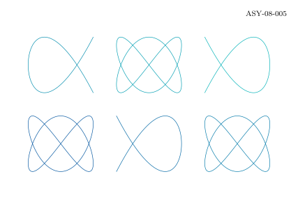
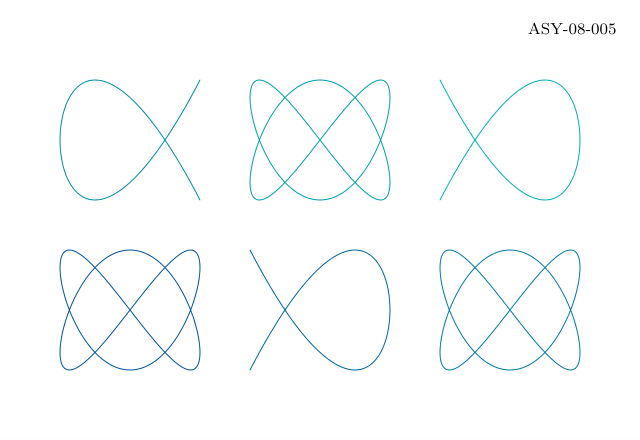
`phase`	Change only the x-coordinate phase.
`Small multiples`	Use the same geometry and scale for every panel.

Complete standalone Asymptote program

settings.tex="pdflatex";
settings.outformat="pdf";
settings.render=0;
settings.prc=false;
settings.v3d=false;
defaultpen(fontsize(10pt));
pen Blue=rgb(0,84/255.0,159/255.0),Teal=rgb(0,177/255.0,183/255.0);
pen Orange=rgb(246/255.0,168/255.0,0),Green=rgb(87/255.0,171/255.0,39/255.0);
pen Grey=gray(.4),Light=gray(.92),Wash=rgb(232/255.0,241/255.0,250/255.0);
string figureID="ASY-08-005";
size(320,220,IgnoreAspect);
fill(box((0,0),(320,220)),white);
// BEGIN DRAWING
import graph;
for(int j=0;j<2;++j) for(int i=0;i<3;++i) {
 real phase=(i+3*j)*pi/6;
 pair f(real t) {return (65+95*i,65+85*j)+(35*sin(2*t+phase),30*cos(3*t));}
 draw(graph(f,0,2*pi,240),interp(Blue,Teal,(i+3*j)/5.0));
}
// END DRAWING
label("ASY-08-005",(310,210),SW,fontsize(8pt));
shipout(figureID);

Download: Asymptote source · SVG figure · Vector PDF · PNG preview

ASY-08-006

Map a grid through the complex square

Asymptote pairs support complex arithmetic. Squaring maps straight coordinate lines into parabolic curves.

Back to figure overview

Asymptote drawing

import graph;
for(int i=-4;i<=4;++i) {
 real a=i/4.0;
 pair f(real t) {return (160,105)+42*(a,t)^2;}
 pair g(real t) {return (160,105)+42*(t,a)^2;}
 draw(graph(f,-1.2,1.2,120),Blue+.7);
 draw(graph(g,-1.2,1.2,120),Teal+.7);
}

Actual output

Map a grid through the complex square — ASY-08-006 · Rendered by Asymptote

Asymptote · exit 0

Native compiler log

Compilation completed successfully. No compiler messages were emitted.

Command or parameter	Meaning
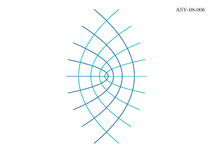
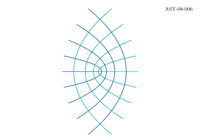
`pair squared`	Use the pair as a complex number.
`Two grid families`	Transform both horizontal and vertical coordinate lines.

Complete standalone Asymptote program

settings.tex="pdflatex";
settings.outformat="pdf";
settings.render=0;
settings.prc=false;
settings.v3d=false;
defaultpen(fontsize(10pt));
pen Blue=rgb(0,84/255.0,159/255.0),Teal=rgb(0,177/255.0,183/255.0);
pen Orange=rgb(246/255.0,168/255.0,0),Green=rgb(87/255.0,171/255.0,39/255.0);
pen Grey=gray(.4),Light=gray(.92),Wash=rgb(232/255.0,241/255.0,250/255.0);
string figureID="ASY-08-006";
size(320,220,IgnoreAspect);
fill(box((0,0),(320,220)),white);
// BEGIN DRAWING
import graph;
for(int i=-4;i<=4;++i) {
 real a=i/4.0;
 pair f(real t) {return (160,105)+42*(a,t)^2;}
 pair g(real t) {return (160,105)+42*(t,a)^2;}
 draw(graph(f,-1.2,1.2,120),Blue+.7);
 draw(graph(g,-1.2,1.2,120),Teal+.7);
}
// END DRAWING
label("ASY-08-006",(310,210),SW,fontsize(8pt));
shipout(figureID);

Download: Asymptote source · SVG figure · Vector PDF · PNG preview

09 · Geometry and diagrams

ASY-09-001

Construct a midpoint and median

A coordinate average locates the midpoint exactly. The median joins that point to the opposite vertex.

Back to figure overview

Asymptote drawing

pair a=(45,45),b=(275,65),c=(155,180),m=(a+b)/2;
filldraw(a--b--c--cycle,Wash,Blue);
draw(c--m,Teal+1.5); dot(m,Orange+5);
label("midpoint",m,S);

Actual output

Construct a midpoint and median — ASY-09-001 · Rendered by Asymptote

Asymptote · exit 0

Native compiler log

Compilation completed successfully. No compiler messages were emitted.

Command or parameter	Meaning
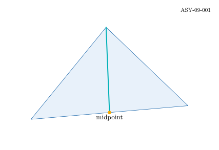
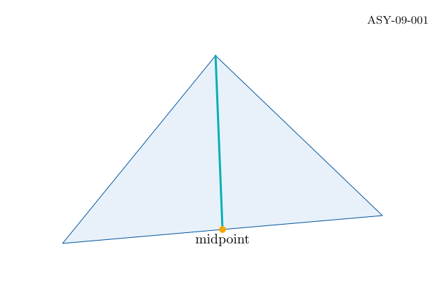
`(a+b)/2`	Compute the midpoint component by component.
`Median`	Connect a vertex to the opposite side midpoint.

Complete standalone Asymptote program

settings.tex="pdflatex";
settings.outformat="pdf";
settings.render=0;
settings.prc=false;
settings.v3d=false;
defaultpen(fontsize(10pt));
pen Blue=rgb(0,84/255.0,159/255.0),Teal=rgb(0,177/255.0,183/255.0);
pen Orange=rgb(246/255.0,168/255.0,0),Green=rgb(87/255.0,171/255.0,39/255.0);
pen Grey=gray(.4),Light=gray(.92),Wash=rgb(232/255.0,241/255.0,250/255.0);
string figureID="ASY-09-001";
size(320,220,IgnoreAspect);
fill(box((0,0),(320,220)),white);
// BEGIN DRAWING
pair a=(45,45),b=(275,65),c=(155,180),m=(a+b)/2;
filldraw(a--b--c--cycle,Wash,Blue);
draw(c--m,Teal+1.5); dot(m,Orange+5);
label("midpoint",m,S);
// END DRAWING
label("ASY-09-001",(310,210),SW,fontsize(8pt));
shipout(figureID);

Download: Asymptote source · SVG figure · Vector PDF · PNG preview

ASY-09-002

Project a point onto a line

The scalar projection determines the perpendicular foot. The right-angle marker is computed from the same unit directions.

Back to figure overview

Asymptote drawing

pair a=(40,55),b=(280,110),p=(215,180);
pair u=unit(b-a),v=(-u.y,u.x);
pair foot=a+dot(p-a,u)*u;
draw(a--b,Blue+1.5); draw(p--foot,Teal+dashed);
draw(foot+8*u--foot+8*u+8*v--foot+8*v,Grey);
dot(p,Orange+4); dot(foot,Orange+4);

Actual output

Project a point onto a line — ASY-09-002 · Rendered by Asymptote

Asymptote · exit 0

Native compiler log

Compilation completed successfully. No compiler messages were emitted.

Command or parameter	Meaning
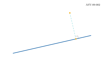
`dot(p-a,u)`	Compute signed distance along the unit direction.
`Perpendicular vector`	Rotate u by ninety degrees.

Complete standalone Asymptote program

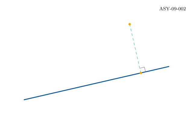
settings.tex="pdflatex";
settings.outformat="pdf";
settings.render=0;
settings.prc=false;
settings.v3d=false;
defaultpen(fontsize(10pt));
pen Blue=rgb(0,84/255.0,159/255.0),Teal=rgb(0,177/255.0,183/255.0);
pen Orange=rgb(246/255.0,168/255.0,0),Green=rgb(87/255.0,171/255.0,39/255.0);
pen Grey=gray(.4),Light=gray(.92),Wash=rgb(232/255.0,241/255.0,250/255.0);
string figureID="ASY-09-002";
size(320,220,IgnoreAspect);
fill(box((0,0),(320,220)),white);
// BEGIN DRAWING
pair a=(40,55),b=(280,110),p=(215,180);
pair u=unit(b-a),v=(-u.y,u.x);
pair foot=a+dot(p-a,u)*u;
draw(a--b,Blue+1.5); draw(p--foot,Teal+dashed);
draw(foot+8*u--foot+8*u+8*v--foot+8*v,Grey);
dot(p,Orange+4); dot(foot,Orange+4);
// END DRAWING
label("ASY-09-002",(310,210),SW,fontsize(8pt));
shipout(figureID);

Download: Asymptote source · SVG figure · Vector PDF · PNG preview

ASY-09-003

Compute a crank and slider

The slider position is solved from the connecting-rod length. Changing the crank angle preserves both link lengths.

Back to figure overview

Asymptote drawing

pair o=(70,105); real r=40,L=135,theta=55;
pair a=o+r*dir(theta);
real dx=sqrt(L^2-(a.y-o.y)^2);
pair b=(a.x+dx,o.y);
draw(circle(o,r),Light+dashed);
draw((30,105)--(290,105),Grey+dashed);
filldraw(box(b+(-14,-12),b+(14,12)),Wash,Blue);
draw(o--a,Blue+4); draw(a--b,Teal+4);
dot(new pair[] {o,a,b},Orange+6);
write("check: rod-length="+(string)abs(b-a));

Actual output

Compute a crank and slider — ASY-09-003 · Rendered by Asymptote

Asymptote · exit 0

Native compiler log

Standard output

check: rod-length=135

Command or parameter	Meaning
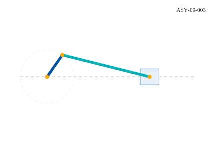
`sqrt constraint`	Solve the right triangle for the horizontal offset.
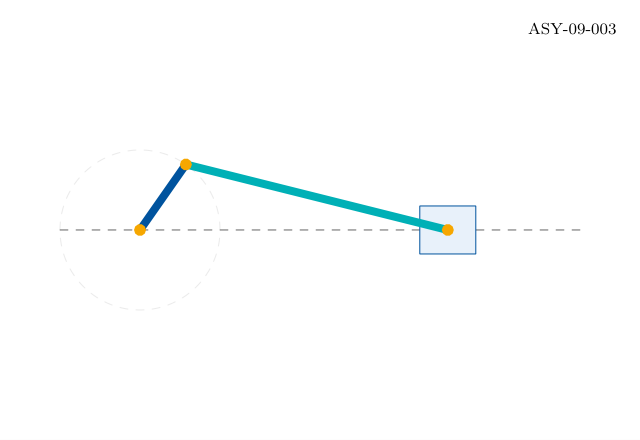
`L=135`	Preserve the connecting-rod length.
`theta`	Crank angle in degrees.

Complete standalone Asymptote program

settings.tex="pdflatex";
settings.outformat="pdf";
settings.render=0;
settings.prc=false;
settings.v3d=false;
defaultpen(fontsize(10pt));
pen Blue=rgb(0,84/255.0,159/255.0),Teal=rgb(0,177/255.0,183/255.0);
pen Orange=rgb(246/255.0,168/255.0,0),Green=rgb(87/255.0,171/255.0,39/255.0);
pen Grey=gray(.4),Light=gray(.92),Wash=rgb(232/255.0,241/255.0,250/255.0);
string figureID="ASY-09-003";
size(320,220,IgnoreAspect);
fill(box((0,0),(320,220)),white);
// BEGIN DRAWING
pair o=(70,105); real r=40,L=135,theta=55;
pair a=o+r*dir(theta);
real dx=sqrt(L^2-(a.y-o.y)^2);
pair b=(a.x+dx,o.y);
draw(circle(o,r),Light+dashed);
draw((30,105)--(290,105),Grey+dashed);
filldraw(box(b+(-14,-12),b+(14,12)),Wash,Blue);
draw(o--a,Blue+4); draw(a--b,Teal+4);
dot(new pair[] {o,a,b},Orange+6);
write("check: rod-length="+(string)abs(b-a));
// END DRAWING
label("ASY-09-003",(310,210),SW,fontsize(8pt));
shipout(figureID);

Download: Asymptote source · SVG figure · Vector PDF · PNG preview

ASY-09-004

Solve a circle intersection

Subtracting the two circle equations gives the common chord location. A square root gives its half-height.

Back to figure overview

Asymptote drawing

pair a=(110,105),b=(210,105); real r=70,d=abs(b-a);
real x=d/2,y=sqrt(r^2-x^2);
pair upper=a+(x,y),lower=a+(x,-y);
draw(circle(a,r),Blue); draw(circle(b,r),Teal);
draw(lower--upper,Orange+2);
dot(new pair[] {upper,lower},Orange+5);

Actual output

Solve a circle intersection — ASY-09-004 · Rendered by Asymptote

Asymptote · exit 0

Native compiler log

Compilation completed successfully. No compiler messages were emitted.

Command or parameter	Meaning
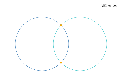
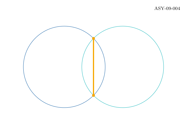
`Equal radii`	The common chord lies midway between centres.
`r^2-x^2`	Compute the squared half-chord length.

Complete standalone Asymptote program

settings.tex="pdflatex";
settings.outformat="pdf";
settings.render=0;
settings.prc=false;
settings.v3d=false;
defaultpen(fontsize(10pt));
pen Blue=rgb(0,84/255.0,159/255.0),Teal=rgb(0,177/255.0,183/255.0);
pen Orange=rgb(246/255.0,168/255.0,0),Green=rgb(87/255.0,171/255.0,39/255.0);
pen Grey=gray(.4),Light=gray(.92),Wash=rgb(232/255.0,241/255.0,250/255.0);
string figureID="ASY-09-004";
size(320,220,IgnoreAspect);
fill(box((0,0),(320,220)),white);
// BEGIN DRAWING
pair a=(110,105),b=(210,105); real r=70,d=abs(b-a);
real x=d/2,y=sqrt(r^2-x^2);
pair upper=a+(x,y),lower=a+(x,-y);
draw(circle(a,r),Blue); draw(circle(b,r),Teal);
draw(lower--upper,Orange+2);
dot(new pair[] {upper,lower},Orange+5);
// END DRAWING
label("ASY-09-004",(310,210),SW,fontsize(8pt));
shipout(figureID);

Download: Asymptote source · SVG figure · Vector PDF · PNG preview

ASY-09-005

Connect nodes at their boundaries

Shorten each connector by the node radius at both ends. The arrows then touch the circles rather than crossing their labels.

Back to figure overview

Asymptote drawing

pair[] p={(60,145),(260,145),(160,55)};
string[] names={"observe","model","test"}; real r=25;
for(int i=0;i<3;++i) {
 int j=(i+1)%3; pair u=unit(p[j]-p[i]);
 draw(p[i]+r*u--p[j]-r*u,Blue,Arrow(5));
}
for(int i=0;i<3;++i) {filldraw(circle(p[i],r),Wash,Teal); label(names[i],p[i]);}

Actual output

Connect nodes at their boundaries — ASY-09-005 · Rendered by Asymptote

Asymptote · exit 0

Native compiler log

Compilation completed successfully. No compiler messages were emitted.

Command or parameter	Meaning
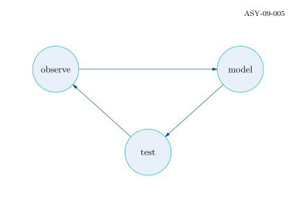
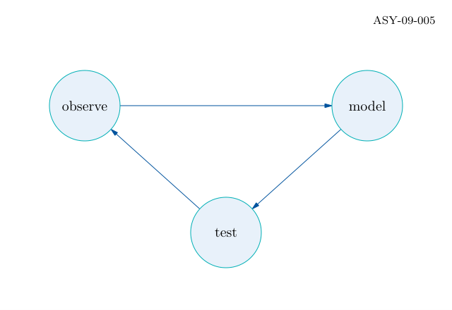
`unit(b-a)`	Find the connector direction.
`Radius offsets`	Place endpoints on circular boundaries.

Complete standalone Asymptote program

settings.tex="pdflatex";
settings.outformat="pdf";
settings.render=0;
settings.prc=false;
settings.v3d=false;
defaultpen(fontsize(10pt));
pen Blue=rgb(0,84/255.0,159/255.0),Teal=rgb(0,177/255.0,183/255.0);
pen Orange=rgb(246/255.0,168/255.0,0),Green=rgb(87/255.0,171/255.0,39/255.0);
pen Grey=gray(.4),Light=gray(.92),Wash=rgb(232/255.0,241/255.0,250/255.0);
string figureID="ASY-09-005";
size(320,220,IgnoreAspect);
fill(box((0,0),(320,220)),white);
// BEGIN DRAWING
pair[] p={(60,145),(260,145),(160,55)};
string[] names={"observe","model","test"}; real r=25;
for(int i=0;i<3;++i) {
 int j=(i+1)%3; pair u=unit(p[j]-p[i]);
 draw(p[i]+r*u--p[j]-r*u,Blue,Arrow(5));
}
for(int i=0;i<3;++i) {filldraw(circle(p[i],r),Wash,Teal); label(names[i],p[i]);}
// END DRAWING
label("ASY-09-005",(310,210),SW,fontsize(8pt));
shipout(figureID);

Download: Asymptote source · SVG figure · Vector PDF · PNG preview

ASY-09-006

Typeset mathematical annotations

TeX handles equations and ordinary prose in one label system. Alignment directions keep text separate from its anchor.

Back to figure overview

Asymptote drawing

draw((45,55)--(275,55)--(275,170)--cycle,Blue+1.5);
label("$a$",(160,55),S); label("$b$",(275,112),E);
label("$c$",(160,112),NW);
label("$a^2+b^2=c^2$",(140,180));
draw((263,55)--(263,67)--(275,67),Grey);

Actual output

Typeset mathematical annotations — ASY-09-006 · Rendered by Asymptote

Asymptote · exit 0

Native compiler log

Compilation completed successfully. No compiler messages were emitted.

Command or parameter	Meaning
`TeX strings`	Use dollar delimiters for mathematics.
`Alignment`	N, S, E and W specify label placement relative to the anchor.

Complete standalone Asymptote program

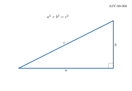
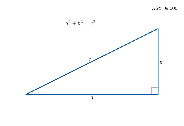
settings.tex="pdflatex";
settings.outformat="pdf";
settings.render=0;
settings.prc=false;
settings.v3d=false;
defaultpen(fontsize(10pt));
pen Blue=rgb(0,84/255.0,159/255.0),Teal=rgb(0,177/255.0,183/255.0);
pen Orange=rgb(246/255.0,168/255.0,0),Green=rgb(87/255.0,171/255.0,39/255.0);
pen Grey=gray(.4),Light=gray(.92),Wash=rgb(232/255.0,241/255.0,250/255.0);
string figureID="ASY-09-006";
size(320,220,IgnoreAspect);
fill(box((0,0),(320,220)),white);
// BEGIN DRAWING
draw((45,55)--(275,55)--(275,170)--cycle,Blue+1.5);
label("$a$",(160,55),S); label("$b$",(275,112),E);
label("$c$",(160,112),NW);
label("$a^2+b^2=c^2$",(140,180));
draw((263,55)--(263,67)--(275,67),Grey);
// END DRAWING
label("ASY-09-006",(310,210),SW,fontsize(8pt));
shipout(figureID);

Download: Asymptote source · SVG figure · Vector PDF · PNG preview

10 · Curves in three dimensions

ASY-10-001

Project a helix into the plane

A triple-valued function defines a spatial curve. Explicit project converts it into a planar path that can be styled with ordinary 2D drawing tools.

Back to figure overview

Asymptote drawing

import graph3;
triple helix(real t) {return (cos(t),sin(t),t/(2*pi));}
projection camera=orthographic(4,6,3);
path p=project(graph(helix,0,6*pi,400),camera);
draw(shift(160,60)*scale(36)*p,Blue+1.5);
draw(shift(160,60)*scale(36)*project(O--3.3*Z,camera),Grey+dashed);

Actual output

Project a helix into the plane — ASY-10-001 · Rendered by Asymptote

Asymptote · exit 0

Native compiler log

Compilation completed successfully. No compiler messages were emitted.

Command or parameter	Meaning
`triple`	Represent a point or vector in three dimensions.
`project(path3,camera)`	Return a 2D path under the chosen projection.

Complete standalone Asymptote program

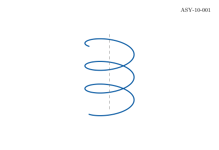
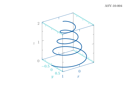
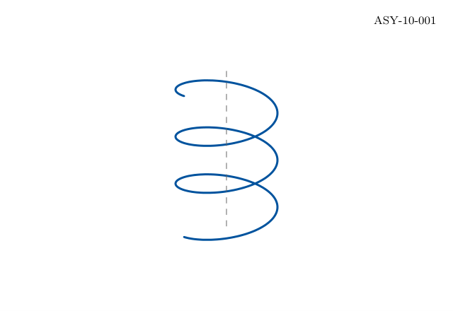
settings.tex="pdflatex";
settings.outformat="pdf";
settings.render=0;
settings.prc=false;
settings.v3d=false;
defaultpen(fontsize(10pt));
pen Blue=rgb(0,84/255.0,159/255.0),Teal=rgb(0,177/255.0,183/255.0);
pen Orange=rgb(246/255.0,168/255.0,0),Green=rgb(87/255.0,171/255.0,39/255.0);
pen Grey=gray(.4),Light=gray(.92),Wash=rgb(232/255.0,241/255.0,250/255.0);
string figureID="ASY-10-001";
size(320,220,IgnoreAspect);
fill(box((0,0),(320,220)),white);
// BEGIN DRAWING
import graph3;
triple helix(real t) {return (cos(t),sin(t),t/(2*pi));}
projection camera=orthographic(4,6,3);
path p=project(graph(helix,0,6*pi,400),camera);
draw(shift(160,60)*scale(36)*p,Blue+1.5);
draw(shift(160,60)*scale(36)*project(O--3.3*Z,camera),Grey+dashed);
// END DRAWING
label("ASY-10-001",(310,210),SW,fontsize(8pt));
shipout(figureID);

Download: Asymptote source · SVG figure · Vector PDF · PNG preview

ASY-10-002

Draw a native spatial helix

The same triple-valued curve is drawn directly as a path3. The native 3D engine handles projection before the result is placed on the page.

Back to figure overview

Compare with ASY-10-001 · Project a helix into the plane.

Asymptote drawing

import graph3;
currentprojection=orthographic(4,6,3);
triple helix(real t) {return (cos(t),sin(t),t/(2*pi));}
draw(graph(helix,0,6*pi,400),Blue+1.5);
draw(O--3.3*Z,Grey+dashed,Arrow3);

Actual output

Draw a native spatial helix — ASY-10-002 · Rendered by Asymptote

Asymptote · exit 0

Native compiler log

Compilation completed successfully. No compiler messages were emitted.

Command or parameter	Meaning
`path3`	Keep the curve in three-dimensional coordinates.
`Arrow3`	Use a spatial arrowhead.
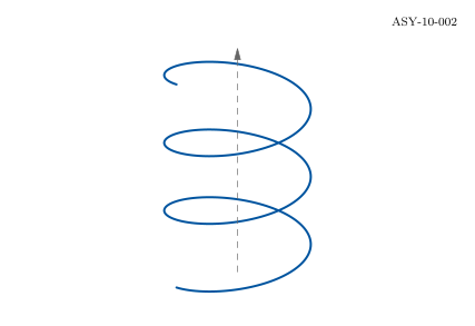
`render=0`	Produce a static vector projection.

Complete standalone Asymptote program

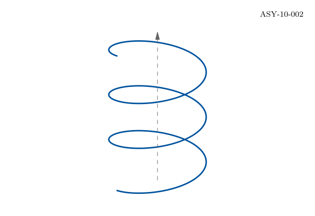
settings.tex="pdflatex";
settings.outformat="pdf";
settings.render=0;
settings.prc=false;
settings.v3d=false;
defaultpen(fontsize(10pt));
pen Blue=rgb(0,84/255.0,159/255.0),Teal=rgb(0,177/255.0,183/255.0);
pen Orange=rgb(246/255.0,168/255.0,0),Green=rgb(87/255.0,171/255.0,39/255.0);
pen Grey=gray(.4),Light=gray(.92),Wash=rgb(232/255.0,241/255.0,250/255.0);
string figureID="ASY-10-002";
size(270,165);
// BEGIN DRAWING
import graph3;
currentprojection=orthographic(4,6,3);
triple helix(real t) {return (cos(t),sin(t),t/(2*pi));}
draw(graph(helix,0,6*pi,400),Blue+1.5);
draw(O--3.3*Z,Grey+dashed,Arrow3);
// END DRAWING
picture drawing=currentpicture;
currentpicture=new picture;
size(320,220,IgnoreAspect);
fill(box((0,0),(320,220)),white);
add(drawing.fit3(),(160,105),align=0);
label("ASY-10-002",(310,210),SW,fontsize(8pt));
shipout(figureID);

Download: Asymptote source · SVG figure · Vector PDF · PNG preview

ASY-10-003

Trace a torus knot

Two angular frequencies wrap a curve around a torus. The source retains its spatial coordinates and a fixed camera.

Back to figure overview

Asymptote drawing

import graph3;
currentprojection=orthographic(4,5,6);
triple knot(real t) {
 return ((2+.65*cos(3*t))*cos(2*t),(2+.65*cos(3*t))*sin(2*t),.65*sin(3*t));
}
draw(graph(knot,0,2*pi,600),Blue+1.5);

Actual output

Trace a torus knot — ASY-10-003 · Rendered by Asymptote

Asymptote · exit 0

Native compiler log

Compilation completed successfully. No compiler messages were emitted.

Command or parameter	Meaning
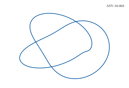
`2 and 3 windings`	Set the two integer frequencies of this torus knot.
`Fixed camera`	Keep comparison and print views reproducible.

Complete standalone Asymptote program

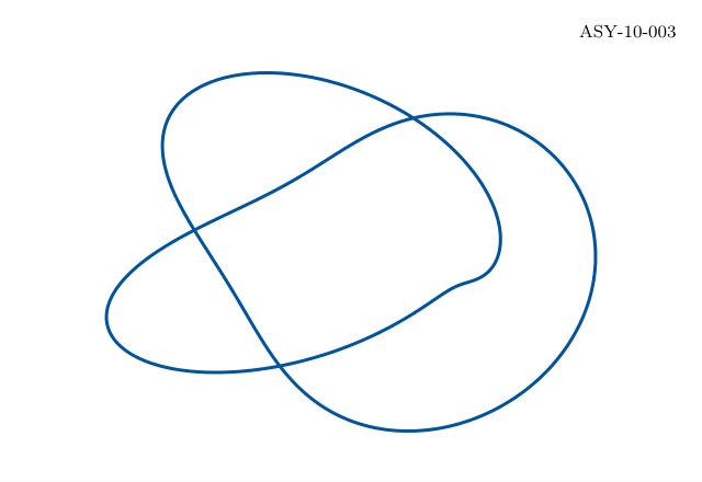
settings.tex="pdflatex";
settings.outformat="pdf";
settings.render=0;
settings.prc=false;
settings.v3d=false;
defaultpen(fontsize(10pt));
pen Blue=rgb(0,84/255.0,159/255.0),Teal=rgb(0,177/255.0,183/255.0);
pen Orange=rgb(246/255.0,168/255.0,0),Green=rgb(87/255.0,171/255.0,39/255.0);
pen Grey=gray(.4),Light=gray(.92),Wash=rgb(232/255.0,241/255.0,250/255.0);
string figureID="ASY-10-003";
size(270,165);
// BEGIN DRAWING
import graph3;
currentprojection=orthographic(4,5,6);
triple knot(real t) {
 return ((2+.65*cos(3*t))*cos(2*t),(2+.65*cos(3*t))*sin(2*t),.65*sin(3*t));
}
draw(graph(knot,0,2*pi,600),Blue+1.5);
// END DRAWING
picture drawing=currentpicture;
currentpicture=new picture;
size(320,220,IgnoreAspect);
fill(box((0,0),(320,220)),white);
add(drawing.fit3(),(160,105),align=0);
label("ASY-10-003",(310,210),SW,fontsize(8pt));
shipout(figureID);

Download: Asymptote source · SVG figure · Vector PDF · PNG preview

ASY-10-004

Place axes around a spatial curve

Axis labels and ticks use native graph3 coordinates. The curve is an explicit damped spiral in space.

Back to figure overview

Asymptote drawing

import graph3;
currentprojection=orthographic(5,7,4);
triple f(real t) {return (exp(-.15*t)*cos(3*t),exp(-.15*t)*sin(3*t),t/4);}
draw(graph(f,0,8,350),Blue+1.5);
xaxis3("$x$",Bounds,Blue,InTicks);
yaxis3("$y$",Bounds,Teal,InTicks);
zaxis3("$z$",Bounds,Grey,InTicks);

Actual output

Place axes around a spatial curve — ASY-10-004 · Rendered by Asymptote

Asymptote · exit 0

Native compiler log

Compilation completed successfully. No compiler messages were emitted.

Command or parameter	Meaning
`Bounds`	Place axes at the spatial bounding box.
`InTicks`	Draw inward tick marks.
`Damping`	Decrease radius as height increases.

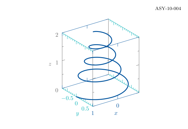
Complete standalone Asymptote program

settings.tex="pdflatex";
settings.outformat="pdf";
settings.render=0;
settings.prc=false;
settings.v3d=false;
defaultpen(fontsize(10pt));
pen Blue=rgb(0,84/255.0,159/255.0),Teal=rgb(0,177/255.0,183/255.0);
pen Orange=rgb(246/255.0,168/255.0,0),Green=rgb(87/255.0,171/255.0,39/255.0);
pen Grey=gray(.4),Light=gray(.92),Wash=rgb(232/255.0,241/255.0,250/255.0);
string figureID="ASY-10-004";
size(270,165);
// BEGIN DRAWING
import graph3;
currentprojection=orthographic(5,7,4);
triple f(real t) {return (exp(-.15*t)*cos(3*t),exp(-.15*t)*sin(3*t),t/4);}
draw(graph(f,0,8,350),Blue+1.5);
xaxis3("$x$",Bounds,Blue,InTicks);
yaxis3("$y$",Bounds,Teal,InTicks);
zaxis3("$z$",Bounds,Grey,InTicks);
// END DRAWING
picture drawing=currentpicture;
currentpicture=new picture;
size(320,220,IgnoreAspect);
fill(box((0,0),(320,220)),white);
add(drawing.fit3(),(160,105),align=0);
label("ASY-10-004",(310,210),SW,fontsize(8pt));
shipout(figureID);

Download: Asymptote source · SVG figure · Vector PDF · PNG preview

ASY-10-005

Compare orthographic and perspective views

The same cube edges are projected twice. Perspective makes parallel depth edges converge; orthographic projection preserves their parallelism.

Back to figure overview

Asymptote drawing

import three;
triple[] v={(-1,-1,-1),(1,-1,-1),(1,1,-1),(-1,1,-1),(-1,-1,1),(1,-1,1),(1,1,1),(-1,1,1)};
for(int k=0;k<2;++k) {
 projection camera=k==0 ? orthographic(4,6,3) : perspective(4,6,3);
 transform T=shift(80+160*k,105)*scale(30);
 for(int i=0;i<4;++i) {
  draw(T*project(v[i]--v[(i+1)%4],camera),Blue);
  draw(T*project(v[i+4]--v[(i+1)%4+4],camera),Blue);
  draw(T*project(v[i]--v[i+4],camera),Teal);
 }
 label(k==0 ? "orthographic" : "perspective",(80+160*k,35));
}

Actual output

Compare orthographic and perspective views — ASY-10-005 · Rendered by Asymptote

Asymptote · exit 0

Native compiler log

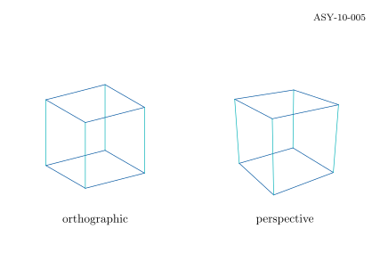
Compilation completed successfully. No compiler messages were emitted.

Command or parameter	Meaning
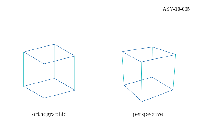
`orthographic`	Remove depth-dependent size change.
`perspective`	Project from a finite camera position.

Complete standalone Asymptote program

settings.tex="pdflatex";
settings.outformat="pdf";
settings.render=0;
settings.prc=false;
settings.v3d=false;
defaultpen(fontsize(10pt));
pen Blue=rgb(0,84/255.0,159/255.0),Teal=rgb(0,177/255.0,183/255.0);
pen Orange=rgb(246/255.0,168/255.0,0),Green=rgb(87/255.0,171/255.0,39/255.0);
pen Grey=gray(.4),Light=gray(.92),Wash=rgb(232/255.0,241/255.0,250/255.0);
string figureID="ASY-10-005";
size(320,220,IgnoreAspect);
fill(box((0,0),(320,220)),white);
// BEGIN DRAWING
import three;
triple[] v={(-1,-1,-1),(1,-1,-1),(1,1,-1),(-1,1,-1),(-1,-1,1),(1,-1,1),(1,1,1),(-1,1,1)};
for(int k=0;k<2;++k) {
 projection camera=k==0 ? orthographic(4,6,3) : perspective(4,6,3);
 transform T=shift(80+160*k,105)*scale(30);
 for(int i=0;i<4;++i) {
  draw(T*project(v[i]--v[(i+1)%4],camera),Blue);
  draw(T*project(v[i+4]--v[(i+1)%4+4],camera),Blue);
  draw(T*project(v[i]--v[i+4],camera),Teal);
 }
 label(k==0 ? "orthographic" : "perspective",(80+160*k,35));
}
// END DRAWING
label("ASY-10-005",(310,210),SW,fontsize(8pt));
shipout(figureID);

Download: Asymptote source · SVG figure · Vector PDF · PNG preview

ASY-10-006

Draw a spatial vector triad

Three arrows and a diagonal vector share the same origin. TeX labels remain attached to their spatial endpoints.

Back to figure overview

Asymptote drawing

import three;
currentprojection=orthographic(4,6,3);
draw(O--X,Blue+1.5,Arrow3);
draw(O--Y,Teal+1.5,Arrow3);
draw(O--Z,Orange+1.5,Arrow3);
draw(O--(1,1,.7),Grey+1.5,Arrow3);
label("$x$",1.2X,S); label("$y$",1.2Y,E); label("$z$",1.1Z,N);

Actual output

Draw a spatial vector triad — ASY-10-006 · Rendered by Asymptote

Asymptote · exit 0

Native compiler log

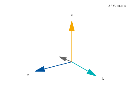
Compilation completed successfully. No compiler messages were emitted.

Command or parameter	Meaning
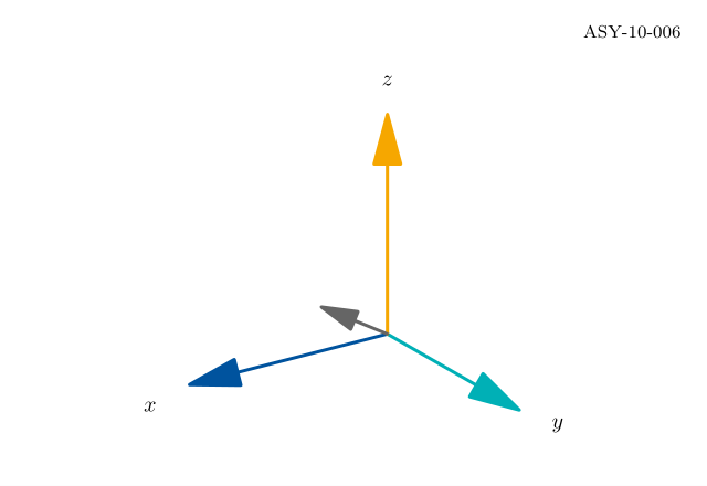
`O, X, Y, Z`	Use standard triples for the origin and coordinate directions.
`Spatial labels`	Place each label in the same coordinate system as its arrow.

Complete standalone Asymptote program

settings.tex="pdflatex";
settings.outformat="pdf";
settings.render=0;
settings.prc=false;
settings.v3d=false;
defaultpen(fontsize(10pt));
pen Blue=rgb(0,84/255.0,159/255.0),Teal=rgb(0,177/255.0,183/255.0);
pen Orange=rgb(246/255.0,168/255.0,0),Green=rgb(87/255.0,171/255.0,39/255.0);
pen Grey=gray(.4),Light=gray(.92),Wash=rgb(232/255.0,241/255.0,250/255.0);
string figureID="ASY-10-006";
size(270,165);
// BEGIN DRAWING
import three;
currentprojection=orthographic(4,6,3);
draw(O--X,Blue+1.5,Arrow3);
draw(O--Y,Teal+1.5,Arrow3);
draw(O--Z,Orange+1.5,Arrow3);
draw(O--(1,1,.7),Grey+1.5,Arrow3);
label("$x$",1.2X,S); label("$y$",1.2Y,E); label("$z$",1.1Z,N);
// END DRAWING
picture drawing=currentpicture;
currentpicture=new picture;
size(320,220,IgnoreAspect);
fill(box((0,0),(320,220)),white);
add(drawing.fit3(),(160,105),align=0);
label("ASY-10-006",(310,210),SW,fontsize(8pt));
shipout(figureID);

Download: Asymptote source · SVG figure · Vector PDF · PNG preview

11 · Surfaces and projections

ASY-11-001

Project a saddle wireframe

Two families of sampled spatial curves describe a hyperbolic paraboloid. Explicit projection keeps every wire visible, including wires behind others.

Back to figure overview

Asymptote drawing

import graph3;
projection camera=orthographic(4,6,4);
transform T=shift(160,105)*scale(48);
for(int i=-8;i<=8;++i) {
 real a=i/8.0;
 triple f(real t) {return (a,t,.6*(a*a-t*t));}
 triple g(real t) {return (t,a,.6*(t*t-a*a));}
 draw(T*project(graph(f,-1,1,60),camera),Blue+.7);
 draw(T*project(graph(g,-1,1,60),camera),Teal+.7);
}

Actual output

Project a saddle wireframe — ASY-11-001 · Rendered by Asymptote

Asymptote · exit 0

Native compiler log

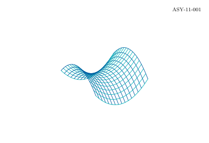
Compilation completed successfully. No compiler messages were emitted.

Command or parameter	Meaning
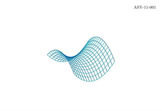
`Wireframe`	Draw both parameter directions.
`No hidden-line solver`	Explicitly projected wires all remain visible.

Complete standalone Asymptote program

settings.tex="pdflatex";
settings.outformat="pdf";
settings.render=0;
settings.prc=false;
settings.v3d=false;
defaultpen(fontsize(10pt));
pen Blue=rgb(0,84/255.0,159/255.0),Teal=rgb(0,177/255.0,183/255.0);
pen Orange=rgb(246/255.0,168/255.0,0),Green=rgb(87/255.0,171/255.0,39/255.0);
pen Grey=gray(.4),Light=gray(.92),Wash=rgb(232/255.0,241/255.0,250/255.0);
string figureID="ASY-11-001";
size(320,220,IgnoreAspect);
fill(box((0,0),(320,220)),white);
// BEGIN DRAWING
import graph3;
projection camera=orthographic(4,6,4);
transform T=shift(160,105)*scale(48);
for(int i=-8;i<=8;++i) {
 real a=i/8.0;
 triple f(real t) {return (a,t,.6*(a*a-t*t));}
 triple g(real t) {return (t,a,.6*(t*t-a*a));}
 draw(T*project(graph(f,-1,1,60),camera),Blue+.7);
 draw(T*project(graph(g,-1,1,60),camera),Teal+.7);
}
// END DRAWING
label("ASY-11-001",(310,210),SW,fontsize(8pt));
shipout(figureID);

Download: Asymptote source · SVG figure · Vector PDF · PNG preview

ASY-11-002

Render a shaded saddle surface

A parametric surface supplies a filled 3D object. The native engine applies lighting and projects the patches to a static vector figure.

Back to figure overview

Compare with ASY-11-001 · Project a saddle wireframe.

Asymptote drawing

import graph3;
currentprojection=orthographic(4,6,4);
triple f(pair t) {return (t.x,t.y,.6*(t.x^2-t.y^2));}
surface s=surface(f,(-1,-1),(1,1),nu=14,nv=14);
draw(s,Blue,meshpen=white+.25);

Actual output

Render a shaded saddle surface — ASY-11-002 · Rendered by Asymptote

Asymptote · exit 0

Native compiler log

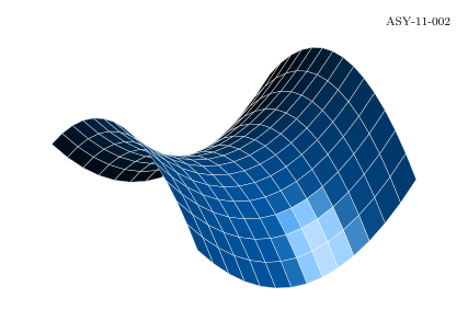
Compilation completed successfully. No compiler messages were emitted.

Command or parameter	Meaning
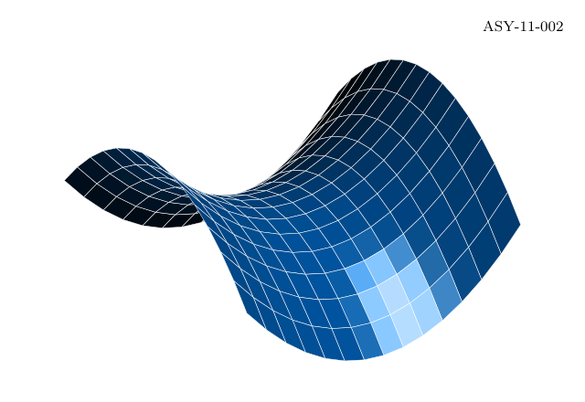
`surface(f,a,b)`	Sample a pair-valued parameter domain into a spatial surface.
`nu / nv`	Set patch counts in the two directions.
`meshpen`	Draw the parameter mesh on the filled surface.

Complete standalone Asymptote program

settings.tex="pdflatex";
settings.outformat="pdf";
settings.render=0;
settings.prc=false;
settings.v3d=false;
defaultpen(fontsize(10pt));
pen Blue=rgb(0,84/255.0,159/255.0),Teal=rgb(0,177/255.0,183/255.0);
pen Orange=rgb(246/255.0,168/255.0,0),Green=rgb(87/255.0,171/255.0,39/255.0);
pen Grey=gray(.4),Light=gray(.92),Wash=rgb(232/255.0,241/255.0,250/255.0);
string figureID="ASY-11-002";
size(270,165);
// BEGIN DRAWING
import graph3;
currentprojection=orthographic(4,6,4);
triple f(pair t) {return (t.x,t.y,.6*(t.x^2-t.y^2));}
surface s=surface(f,(-1,-1),(1,1),nu=14,nv=14);
draw(s,Blue,meshpen=white+.25);
// END DRAWING
picture drawing=currentpicture;
currentpicture=new picture;
size(320,220,IgnoreAspect);
fill(box((0,0),(320,220)),white);
add(drawing.fit3(),(160,105),align=0);
label("ASY-11-002",(310,210),SW,fontsize(8pt));
shipout(figureID);

Download: Asymptote source · SVG figure · Vector PDF · PNG preview

ASY-11-003

Make a sphere from angular parameters

Longitude and latitude map a rectangular parameter domain onto a sphere. A fixed camera and mesh make the coordinate construction visible.

Back to figure overview

Asymptote drawing

import graph3;
currentprojection=orthographic(4,6,3);
triple spherepoint(pair uv) {
 return (cos(uv.x)*cos(uv.y),sin(uv.x)*cos(uv.y),sin(uv.y));
}
surface s=surface(spherepoint,(0,-pi/2),(2*pi,pi/2),nu=24,nv=12);
draw(s,Teal,meshpen=white+.25);

Actual output

Make a sphere from angular parameters — ASY-11-003 · Rendered by Asymptote

Asymptote · exit 0

Native compiler log

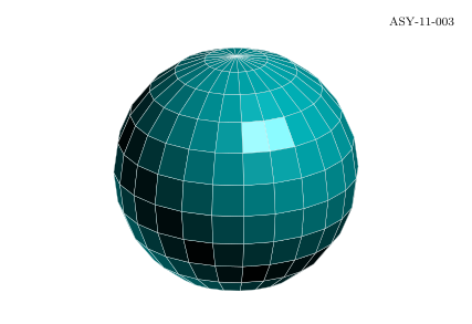
Compilation completed successfully. No compiler messages were emitted.

Command or parameter	Meaning
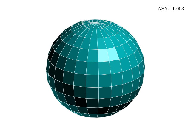
`Angular coordinates`	Use radians for both parameters.
`Latitude poles`	The horizontal radius vanishes at plus or minus pi/2.

Complete standalone Asymptote program

settings.tex="pdflatex";
settings.outformat="pdf";
settings.render=0;
settings.prc=false;
settings.v3d=false;
defaultpen(fontsize(10pt));
pen Blue=rgb(0,84/255.0,159/255.0),Teal=rgb(0,177/255.0,183/255.0);
pen Orange=rgb(246/255.0,168/255.0,0),Green=rgb(87/255.0,171/255.0,39/255.0);
pen Grey=gray(.4),Light=gray(.92),Wash=rgb(232/255.0,241/255.0,250/255.0);
string figureID="ASY-11-003";
size(270,165);
// BEGIN DRAWING
import graph3;
currentprojection=orthographic(4,6,3);
triple spherepoint(pair uv) {
 return (cos(uv.x)*cos(uv.y),sin(uv.x)*cos(uv.y),sin(uv.y));
}
surface s=surface(spherepoint,(0,-pi/2),(2*pi,pi/2),nu=24,nv=12);
draw(s,Teal,meshpen=white+.25);
// END DRAWING
picture drawing=currentpicture;
currentpicture=new picture;
size(320,220,IgnoreAspect);
fill(box((0,0),(320,220)),white);
add(drawing.fit3(),(160,105),align=0);
label("ASY-11-003",(310,210),SW,fontsize(8pt));
shipout(figureID);

Download: Asymptote source · SVG figure · Vector PDF · PNG preview

ASY-11-004

Parameterize a torus surface

Two periodic angles describe a tube wrapped around a larger circle. The major radius and tube radius are independent.

Back to figure overview

Asymptote drawing

import graph3;
currentprojection=orthographic(5,6,4);
triple torus(pair uv) {
 real R=2,r=.65;
 return ((R+r*cos(uv.y))*cos(uv.x),(R+r*cos(uv.y))*sin(uv.x),r*sin(uv.y));
}
draw(surface(torus,(0,0),(2*pi,2*pi),nu=30,nv=14),Blue,meshpen=white+.2);

Actual output

Parameterize a torus surface — ASY-11-004 · Rendered by Asymptote

Asymptote · exit 0

Native compiler log

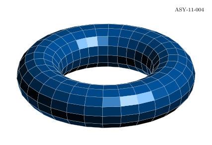
Compilation completed successfully. No compiler messages were emitted.

Command or parameter	Meaning
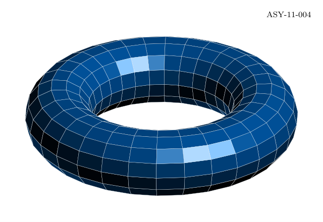
`R=2`	Set distance from the centre to the tube centre.
`r=.65`	Set the tube radius.
`Periodic domain`	Both angles cover one full turn.

Complete standalone Asymptote program

settings.tex="pdflatex";
settings.outformat="pdf";
settings.render=0;
settings.prc=false;
settings.v3d=false;
defaultpen(fontsize(10pt));
pen Blue=rgb(0,84/255.0,159/255.0),Teal=rgb(0,177/255.0,183/255.0);
pen Orange=rgb(246/255.0,168/255.0,0),Green=rgb(87/255.0,171/255.0,39/255.0);
pen Grey=gray(.4),Light=gray(.92),Wash=rgb(232/255.0,241/255.0,250/255.0);
string figureID="ASY-11-004";
size(270,165);
// BEGIN DRAWING
import graph3;
currentprojection=orthographic(5,6,4);
triple torus(pair uv) {
 real R=2,r=.65;
 return ((R+r*cos(uv.y))*cos(uv.x),(R+r*cos(uv.y))*sin(uv.x),r*sin(uv.y));
}
draw(surface(torus,(0,0),(2*pi,2*pi),nu=30,nv=14),Blue,meshpen=white+.2);
// END DRAWING
picture drawing=currentpicture;
currentpicture=new picture;
size(320,220,IgnoreAspect);
fill(box((0,0),(320,220)),white);
add(drawing.fit3(),(160,105),align=0);
label("ASY-11-004",(310,210),SW,fontsize(8pt));
shipout(figureID);

Download: Asymptote source · SVG figure · Vector PDF · PNG preview

ASY-11-005

Revolve a profile around an axis

A height-dependent radius creates a surface of revolution. This model uses a smooth analytic profile rather than imported mesh data.

Back to figure overview

Asymptote drawing

import graph3;
currentprojection=orthographic(5,7,3);
triple vase(pair uv) {
 real r=.65+.22*cos(2*pi*uv.y)+.1*uv.y;
 return (r*cos(uv.x),r*sin(uv.x),2*uv.y);
}
draw(surface(vase,(0,0),(2*pi,1),nu=28,nv=16),Teal,meshpen=white+.2);

Actual output

ASY-11-005 · Rendered by Asymptote

Asymptote · exit 0

Native compiler log

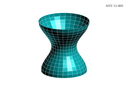
Compilation completed successfully. No compiler messages were emitted.

Command or parameter	Meaning
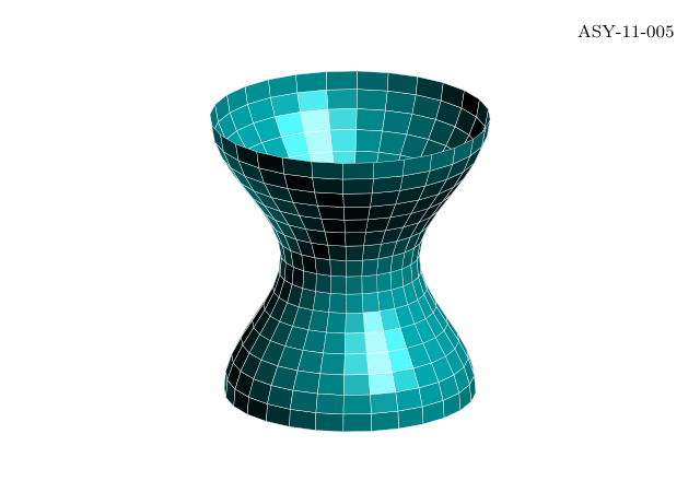
`uv.x`	Angular position around the axis.
`uv.y`	Normalized height between zero and one.
`Profile`	Use one formula for radius as a function of height.

Complete standalone Asymptote program

settings.tex="pdflatex";
settings.outformat="pdf";
settings.render=0;
settings.prc=false;
settings.v3d=false;
defaultpen(fontsize(10pt));
pen Blue=rgb(0,84/255.0,159/255.0),Teal=rgb(0,177/255.0,183/255.0);
pen Orange=rgb(246/255.0,168/255.0,0),Green=rgb(87/255.0,171/255.0,39/255.0);
pen Grey=gray(.4),Light=gray(.92),Wash=rgb(232/255.0,241/255.0,250/255.0);
string figureID="ASY-11-005";
size(270,165);
// BEGIN DRAWING
import graph3;
currentprojection=orthographic(5,7,3);
triple vase(pair uv) {
 real r=.65+.22*cos(2*pi*uv.y)+.1*uv.y;
 return (r*cos(uv.x),r*sin(uv.x),2*uv.y);
}
draw(surface(vase,(0,0),(2*pi,1),nu=28,nv=16),Teal,meshpen=white+.2);
// END DRAWING
picture drawing=currentpicture;
currentpicture=new picture;
size(320,220,IgnoreAspect);
fill(box((0,0),(320,220)),white);
add(drawing.fit3(),(160,105),align=0);
label("ASY-11-005",(310,210),SW,fontsize(8pt));
shipout(figureID);

Download: Asymptote source · SVG figure · Vector PDF · PNG preview

ASY-11-006

Explain a cube with explicit faces

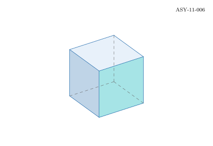
Three selected faces and twelve edges make the projection readable. Hidden edges are styled manually for this chosen view; this is not an automatic visibility algorithm.

Back to figure overview

Asymptote drawing

import three;
projection camera=orthographic(4,6,4);
pair P(triple v) {return (160,105)+40*project(v,camera);}
triple[] v={(-1,-1,-1),(1,-1,-1),(1,1,-1),(-1,1,-1),(-1,-1,1),(1,-1,1),(1,1,1),(-1,1,1)};
fill(P(v[4])--P(v[5])--P(v[6])--P(v[7])--cycle,Wash);
fill(P(v[1])--P(v[2])--P(v[6])--P(v[5])--cycle,interp(white,Blue,.25));
fill(P(v[2])--P(v[3])--P(v[7])--P(v[6])--cycle,interp(white,Teal,.35));
for(int i=0;i<4;++i) {
 draw(P(v[i])--P(v[(i+1)%4]),i==0 || i==3 ? Grey+dashed : Blue);
 draw(P(v[i+4])--P(v[(i+1)%4+4]),Blue);
 draw(P(v[i])--P(v[i+4]),i==0 ? Grey+dashed : Blue);
}

Actual output

Explain a cube with explicit faces — ASY-11-006 · Rendered by Asymptote

Asymptote · exit 0

Native compiler log

Compilation completed successfully. No compiler messages were emitted.

Command or parameter	Meaning
`Explicit faces`	Choose and fill three faces for the fixed camera.
`Hidden edges`	Use dashed pens for the manually identified hidden edges.

Complete standalone Asymptote program

settings.tex="pdflatex";
settings.outformat="pdf";
settings.render=0;
settings.prc=false;
settings.v3d=false;
defaultpen(fontsize(10pt));
pen Blue=rgb(0,84/255.0,159/255.0),Teal=rgb(0,177/255.0,183/255.0);
pen Orange=rgb(246/255.0,168/255.0,0),Green=rgb(87/255.0,171/255.0,39/255.0);
pen Grey=gray(.4),Light=gray(.92),Wash=rgb(232/255.0,241/255.0,250/255.0);
string figureID="ASY-11-006";
size(320,220,IgnoreAspect);
fill(box((0,0),(320,220)),white);
// BEGIN DRAWING
import three;
projection camera=orthographic(4,6,4);
pair P(triple v) {return (160,105)+40*project(v,camera);}
triple[] v={(-1,-1,-1),(1,-1,-1),(1,1,-1),(-1,1,-1),(-1,-1,1),(1,-1,1),(1,1,1),(-1,1,1)};
fill(P(v[4])--P(v[5])--P(v[6])--P(v[7])--cycle,Wash);
fill(P(v[1])--P(v[2])--P(v[6])--P(v[5])--cycle,interp(white,Blue,.25));
fill(P(v[2])--P(v[3])--P(v[7])--P(v[6])--cycle,interp(white,Teal,.35));
for(int i=0;i<4;++i) {
 draw(P(v[i])--P(v[(i+1)%4]),i==0 || i==3 ? Grey+dashed : Blue);
 draw(P(v[i+4])--P(v[(i+1)%4+4]),Blue);
 draw(P(v[i])--P(v[i+4]),i==0 ? Grey+dashed : Blue);
}
// END DRAWING
label("ASY-11-006",(310,210),SW,fontsize(8pt));
shipout(figureID);

Download: Asymptote source · SVG figure · Vector PDF · PNG preview

12 · Composition and publication

ASY-12-001

Clip a picture without editing its paths

A picture stores many drawing operations. clip changes their visibility while preserving the original line definitions.

Back to figure overview

Asymptote drawing

picture waves;
for(int j=-4;j<=16;++j) {
 path p=(0,12*j)..(80,12*j+18)..(160,12*j)..(240,12*j+18)..(320,12*j);
 draw(waves,p,Blue+.7);
}
path boundary=circle((160,105),80);
clip(waves,boundary); add(waves);
draw(boundary,Grey);

Actual output

Clip a picture without editing its paths — ASY-12-001 · Rendered by Asymptote

Asymptote · exit 0

Native compiler log

Compilation completed successfully. No compiler messages were emitted.

Command or parameter	Meaning
`picture`	Collect drawing operations before composition.
`clip`	Keep only the portion inside a closed path.

Complete standalone Asymptote program

settings.tex="pdflatex";
settings.outformat="pdf";
settings.render=0;
settings.prc=false;
settings.v3d=false;
defaultpen(fontsize(10pt));
pen Blue=rgb(0,84/255.0,159/255.0),Teal=rgb(0,177/255.0,183/255.0);
pen Orange=rgb(246/255.0,168/255.0,0),Green=rgb(87/255.0,171/255.0,39/255.0);
pen Grey=gray(.4),Light=gray(.92),Wash=rgb(232/255.0,241/255.0,250/255.0);
string figureID="ASY-12-001";
size(320,220,IgnoreAspect);
fill(box((0,0),(320,220)),white);
// BEGIN DRAWING
picture waves;
for(int j=-4;j<=16;++j) {
 path p=(0,12*j)..(80,12*j+18)..(160,12*j)..(240,12*j+18)..(320,12*j);
 draw(waves,p,Blue+.7);
}
path boundary=circle((160,105),80);
clip(waves,boundary); add(waves);
draw(boundary,Grey);
// END DRAWING
label("ASY-12-001",(310,210),SW,fontsize(8pt));
shipout(figureID);

Download: Asymptote source · SVG figure · Vector PDF · PNG preview

ASY-12-002

Compose independently scaled panels

Separate pictures can use different coordinate systems. Fitted frames are placed explicitly on the common page canvas.

Back to figure overview

Asymptote drawing

import graph;
picture a,b; size(a,120,110); size(b,120,110);
draw(a,graph(sin,0,2*pi),Blue+1.2);
xaxis(a,"$x$",Bottom,Ticks); yaxis(a,"$\sin x$",Left,Ticks);
real f(real x) {return exp(-x);}
draw(b,graph(f,0,4),Teal+1.2);
xaxis(b,"$x$",Bottom,Ticks); yaxis(b,"$e^{-x}$",Left,Ticks);
add(a.fit(),(80,105),align=0); add(b.fit(),(240,105),align=0);
label("(a)",(80,185)); label("(b)",(240,185));

Actual output

Compose independently scaled panels — ASY-12-002 · Rendered by Asymptote

Asymptote · exit 0

Native compiler log

Compilation completed successfully. No compiler messages were emitted.

Command or parameter	Meaning
`size(picture,w,h)`	Scale each subplot independently.
`fit()`	Convert a picture to a physical-size frame.
`add(frame,position)`	Place the fitted result on the common canvas.

Complete standalone Asymptote program

settings.tex="pdflatex";
settings.outformat="pdf";
settings.render=0;
settings.prc=false;
settings.v3d=false;
defaultpen(fontsize(10pt));
pen Blue=rgb(0,84/255.0,159/255.0),Teal=rgb(0,177/255.0,183/255.0);
pen Orange=rgb(246/255.0,168/255.0,0),Green=rgb(87/255.0,171/255.0,39/255.0);
pen Grey=gray(.4),Light=gray(.92),Wash=rgb(232/255.0,241/255.0,250/255.0);
string figureID="ASY-12-002";
size(320,220,IgnoreAspect);
fill(box((0,0),(320,220)),white);
// BEGIN DRAWING
import graph;
picture a,b; size(a,120,110); size(b,120,110);
draw(a,graph(sin,0,2*pi),Blue+1.2);
xaxis(a,"$x$",Bottom,Ticks); yaxis(a,"$\sin x$",Left,Ticks);
real f(real x) {return exp(-x);}
draw(b,graph(f,0,4),Teal+1.2);
xaxis(b,"$x$",Bottom,Ticks); yaxis(b,"$e^{-x}$",Left,Ticks);
add(a.fit(),(80,105),align=0); add(b.fit(),(240,105),align=0);
label("(a)",(80,185)); label("(b)",(240,185));
// END DRAWING
label("ASY-12-002",(310,210),SW,fontsize(8pt));
shipout(figureID);

Download: Asymptote source · SVG figure · Vector PDF · PNG preview

ASY-12-003

Add uncertainty bars and a legend

The intervals are supplied synthetic error extents. Caps, points and legend samples use the same pens as their plotted counterparts.

Back to figure overview

Asymptote drawing

real xmin=0,xmax=5,ymin=0,ymax=8;
pair P(real x,real y) {return (45+245*(x-xmin)/(xmax-xmin),35+145*(y-ymin)/(ymax-ymin));}
for(int i=0;i<=4;++i) {
 real x=xmin+i*(xmax-xmin)/4, y=ymin+i*(ymax-ymin)/4;
 draw(P(x,ymin)--P(x,ymax),Light);
 draw(P(xmin,y)--P(xmax,y),Light);
 label(format("$%.3g$",x),P(x,ymin),S);
 label(format("$%.3g$",y),P(xmin,y),W);
}
draw(P(xmin,ymax)--P(xmin,ymin)--P(xmax,ymin),Grey);
real[] y={2,4,3.5,6},e={.6,.8,.5,1};
for(int i=0;i<y.length;++i) {
 draw(P(i+1,y[i]-e[i])--P(i+1,y[i]+e[i]),Blue,Bars(4));
 dot(P(i+1,y[i]),Orange+5);
}
draw((130,195)--(150,195),Blue,Bars(4)); label("supplied interval",(155,195),E);

Actual output

Add uncertainty bars and a legend — ASY-12-003 · Rendered by Asymptote

Asymptote · exit 0

Native compiler log

Compilation completed successfully. No compiler messages were emitted.

Command or parameter	Meaning
`Supplied intervals`	The example does not infer a confidence level.
`Bars(4)`	Use physical-size end caps.
`Legend sample`	Reuse the actual plotted styling.

Complete standalone Asymptote program

settings.tex="pdflatex";
settings.outformat="pdf";
settings.render=0;
settings.prc=false;
settings.v3d=false;
defaultpen(fontsize(10pt));
pen Blue=rgb(0,84/255.0,159/255.0),Teal=rgb(0,177/255.0,183/255.0);
pen Orange=rgb(246/255.0,168/255.0,0),Green=rgb(87/255.0,171/255.0,39/255.0);
pen Grey=gray(.4),Light=gray(.92),Wash=rgb(232/255.0,241/255.0,250/255.0);
string figureID="ASY-12-003";
size(320,220,IgnoreAspect);
fill(box((0,0),(320,220)),white);
// BEGIN DRAWING
real xmin=0,xmax=5,ymin=0,ymax=8;
pair P(real x,real y) {return (45+245*(x-xmin)/(xmax-xmin),35+145*(y-ymin)/(ymax-ymin));}
for(int i=0;i<=4;++i) {
 real x=xmin+i*(xmax-xmin)/4, y=ymin+i*(ymax-ymin)/4;
 draw(P(x,ymin)--P(x,ymax),Light);
 draw(P(xmin,y)--P(xmax,y),Light);
 label(format("$%.3g$",x),P(x,ymin),S);
 label(format("$%.3g$",y),P(xmin,y),W);
}
draw(P(xmin,ymax)--P(xmin,ymin)--P(xmax,ymin),Grey);
real[] y={2,4,3.5,6},e={.6,.8,.5,1};
for(int i=0;i<y.length;++i) {
 draw(P(i+1,y[i]-e[i])--P(i+1,y[i]+e[i]),Blue,Bars(4));
 dot(P(i+1,y[i]),Orange+5);
}
draw((130,195)--(150,195),Blue,Bars(4)); label("supplied interval",(155,195),E);
// END DRAWING
label("ASY-12-003",(310,210),SW,fontsize(8pt));
shipout(figureID);

Download: Asymptote source · SVG figure · Vector PDF · PNG preview

ASY-12-004

Measure and frame a TeX label

A label is a fitted object with physical dimensions. bbox creates a frame around its typeset contents.

Back to figure overview

Asymptote drawing

picture text;
label(text,"$\displaystyle \int_0^\pi \sin x\,dx=2$",(0,0));
frame f=bbox(text,6,Blue,Fill(Wash));
add(f,(160,105),align=0);

Actual output

Measure and frame a TeX label — ASY-12-004 · Rendered by Asymptote

Asymptote · exit 0

Native compiler log

Compilation completed successfully. No compiler messages were emitted.

Command or parameter	Meaning
`bbox`	Construct a fitted frame around typeset content.
`Padding 6`	Leave six physical points around the label.
`Fill(Wash)`	Give the frame an opaque background.

Complete standalone Asymptote program

settings.tex="pdflatex";
settings.outformat="pdf";
settings.render=0;
settings.prc=false;
settings.v3d=false;
defaultpen(fontsize(10pt));
pen Blue=rgb(0,84/255.0,159/255.0),Teal=rgb(0,177/255.0,183/255.0);
pen Orange=rgb(246/255.0,168/255.0,0),Green=rgb(87/255.0,171/255.0,39/255.0);
pen Grey=gray(.4),Light=gray(.92),Wash=rgb(232/255.0,241/255.0,250/255.0);
string figureID="ASY-12-004";
size(320,220,IgnoreAspect);
fill(box((0,0),(320,220)),white);
// BEGIN DRAWING
picture text;
label(text,"$\displaystyle \int_0^\pi \sin x\,dx=2$",(0,0));
frame f=bbox(text,6,Blue,Fill(Wash));
add(f,(160,105),align=0);
// END DRAWING
label("ASY-12-004",(310,210),SW,fontsize(8pt));
shipout(figureID);

Download: Asymptote source · SVG figure · Vector PDF · PNG preview

ASY-12-005

Separate logical and physical sizes

The fitted geometry can grow while pen widths and text sizes remain physical. Two frames of the same motif show the distinction.

Back to figure overview

Asymptote drawing

picture a,b;
path motif=(0,0)..(1,1)..(2,0);
size(a,85,65); size(b,145,110);
draw(a,motif,Blue+1.5); draw(b,motif,Blue+1.5);
label(a,"small",(1,0),S,fontsize(10pt));
label(b,"large",(1,0),S,fontsize(10pt));
add(a.fit(),(80,105),align=0); add(b.fit(),(230,105),align=0);

Actual output

Separate logical and physical sizes — ASY-12-005 · Rendered by Asymptote

Asymptote · exit 0

Native compiler log

Compilation completed successfully. No compiler messages were emitted.

Command or parameter	Meaning
`size`	Choose the fitted geometric dimensions.
`Physical pens`	Line width remains 1.5 points in both pictures.
`fontsize`	Keep text at ten points in both pictures.

Complete standalone Asymptote program

settings.tex="pdflatex";
settings.outformat="pdf";
settings.render=0;
settings.prc=false;
settings.v3d=false;
defaultpen(fontsize(10pt));
pen Blue=rgb(0,84/255.0,159/255.0),Teal=rgb(0,177/255.0,183/255.0);
pen Orange=rgb(246/255.0,168/255.0,0),Green=rgb(87/255.0,171/255.0,39/255.0);
pen Grey=gray(.4),Light=gray(.92),Wash=rgb(232/255.0,241/255.0,250/255.0);
string figureID="ASY-12-005";
size(320,220,IgnoreAspect);
fill(box((0,0),(320,220)),white);
// BEGIN DRAWING
picture a,b;
path motif=(0,0)..(1,1)..(2,0);
size(a,85,65); size(b,145,110);
draw(a,motif,Blue+1.5); draw(b,motif,Blue+1.5);
label(a,"small",(1,0),S,fontsize(10pt));
label(b,"large",(1,0),S,fontsize(10pt));
add(a.fit(),(80,105),align=0); add(b.fit(),(230,105),align=0);
// END DRAWING
label("ASY-12-005",(310,210),SW,fontsize(8pt));
shipout(figureID);

Download: Asymptote source · SVG figure · Vector PDF · PNG preview

ASY-12-006

Combine a function, tangent and area

A finished plot combines several independent encodings. The tangent uses the analytic derivative; the shaded area is an explicit interval under the function.

Back to figure overview

Asymptote drawing

real xmin=0,xmax=6,ymin=-1.5,ymax=1.5;
pair P(real x,real y) {return (45+245*(x-xmin)/(xmax-xmin),35+145*(y-ymin)/(ymax-ymin));}
for(int i=0;i<=4;++i) {
 real x=xmin+i*(xmax-xmin)/4, y=ymin+i*(ymax-ymin)/4;
 draw(P(x,ymin)--P(x,ymax),Light);
 draw(P(xmin,y)--P(xmax,y),Light);
 label(format("$%.3g$",x),P(x,ymin),S);
 label(format("$%.3g$",y),P(xmin,y),W);
}
draw(P(xmin,ymax)--P(xmin,ymin)--P(xmax,ymin),Grey);
import graph;
pair f(real x) {return P(x,sin(x));}
path p=graph(f,0,6,200),area=graph(f,1,3,80);
fill(area--P(3,0)--P(1,0)--cycle,Wash); draw(p,Blue+1.5);
real a=2,slope=cos(a);
draw(P(1,sin(a)-slope)--P(3,sin(a)+slope),Orange+1.5);
dot(P(a,sin(a)),Teal+5);
label("tangent",P(2.8,1.1),Orange);
write("check: tangent-slope="+(string)slope);

Actual output

Combine a function, tangent and area — ASY-12-006 · Rendered by Asymptote

Asymptote · exit 0

Native compiler log

Standard output

check: tangent-slope=-0.416146836547142

Command or parameter	Meaning
`Analytic derivative`	The sine derivative is cosine, using radians.
`Shaded interval`	Fill only between x=1 and x=3 and the zero baseline.
`One coordinate map`	Use the same P function for every layer.

Complete standalone Asymptote program

settings.tex="pdflatex";
settings.outformat="pdf";
settings.render=0;
settings.prc=false;
settings.v3d=false;
defaultpen(fontsize(10pt));
pen Blue=rgb(0,84/255.0,159/255.0),Teal=rgb(0,177/255.0,183/255.0);
pen Orange=rgb(246/255.0,168/255.0,0),Green=rgb(87/255.0,171/255.0,39/255.0);
pen Grey=gray(.4),Light=gray(.92),Wash=rgb(232/255.0,241/255.0,250/255.0);
string figureID="ASY-12-006";
size(320,220,IgnoreAspect);
fill(box((0,0),(320,220)),white);
// BEGIN DRAWING
real xmin=0,xmax=6,ymin=-1.5,ymax=1.5;
pair P(real x,real y) {return (45+245*(x-xmin)/(xmax-xmin),35+145*(y-ymin)/(ymax-ymin));}
for(int i=0;i<=4;++i) {
 real x=xmin+i*(xmax-xmin)/4, y=ymin+i*(ymax-ymin)/4;
 draw(P(x,ymin)--P(x,ymax),Light);
 draw(P(xmin,y)--P(xmax,y),Light);
 label(format("$%.3g$",x),P(x,ymin),S);
 label(format("$%.3g$",y),P(xmin,y),W);
}
draw(P(xmin,ymax)--P(xmin,ymin)--P(xmax,ymin),Grey);
import graph;
pair f(real x) {return P(x,sin(x));}
path p=graph(f,0,6,200),area=graph(f,1,3,80);
fill(area--P(3,0)--P(1,0)--cycle,Wash); draw(p,Blue+1.5);
real a=2,slope=cos(a);
draw(P(1,sin(a)-slope)--P(3,sin(a)+slope),Orange+1.5);
dot(P(a,sin(a)),Teal+5);
label("tangent",P(2.8,1.1),Orange);
write("check: tangent-slope="+(string)slope);
// END DRAWING
label("ASY-12-006",(310,210),SW,fontsize(8pt));
shipout(figureID);

Download: Asymptote source · SVG figure · Vector PDF · PNG preview

Example and command index

ASY-01-001 · Join two points
ASY-01-002 · Build a polyline
ASY-01-003 · Close and fill a region
ASY-01-004 · Make coordinates visible
ASY-01-005 · Draw circles and boxes
ASY-01-006 · Annotate direction and distance
ASY-02-001 · Interpolate a smooth path
ASY-02-002 · Expose Bezier controls
ASY-02-003 · Constrain endpoint directions
ASY-02-004 · Compare curve tension
ASY-02-005 · Sample a path by arc length
ASY-02-006 · Inspect tangents on a closed path
ASY-03-001 · Compare stroke weights
ASY-03-002 · Compare dash patterns
ASY-03-003 · Interpolate a colour ramp
ASY-03-004 · Transform a reusable motif
ASY-03-005 · See why transform order matters
ASY-03-006 · Reflect and shear geometry
ASY-04-001 · Use arrays as drawing data
ASY-04-002 · Write a pair-valued function
ASY-04-003 · Make a drawing procedure
ASY-04-004 · Use a structure for related values
ASY-04-005 · Distinguish a branch from a loop
ASY-04-006 · Check a numeric calculation in the program
ASY-05-001 · Plot a function and its derivative
ASY-05-002 · Fill the area between functions
ASY-05-003 · Choose logarithmic coordinates
ASY-05-004 · Draw a parametric Lissajous curve
ASY-05-005 · Draw a five-petal polar rose
ASY-05-006 · Estimate an integral with trapezoids
ASY-06-001 · Build bars from an array
ASY-06-002 · Fit a line to observed pairs
ASY-06-003 · Bin raw data into a histogram
ASY-06-004 · Calculate an empirical distribution
ASY-06-005 · Construct a box plot from observations
ASY-06-006 · Estimate a violin density
ASY-07-001 · Draw quadratic level sets
ASY-07-002 · Distinguish positive and negative contours
ASY-07-003 · Colour a triangulated field
ASY-07-004 · Normalize a rotational vector field
ASY-07-005 · Preserve vector magnitudes
ASY-07-006 · Integrate approximate streamlines
ASY-08-001 · Subdivide a triangle recursively
ASY-08-002 · Build a rosette from one petal
ASY-08-003 · Reveal a moire pattern
ASY-08-004 · Draw a logarithmic spiral
ASY-08-005 · Compare phase-shifted trajectories
ASY-08-006 · Map a grid through the complex square
ASY-09-001 · Construct a midpoint and median
ASY-09-002 · Project a point onto a line
ASY-09-003 · Compute a crank and slider
ASY-09-004 · Solve a circle intersection
ASY-09-005 · Connect nodes at their boundaries
ASY-09-006 · Typeset mathematical annotations
ASY-10-001 · Project a helix into the plane
ASY-10-002 · Draw a native spatial helix
ASY-10-003 · Trace a torus knot
ASY-10-004 · Place axes around a spatial curve
ASY-10-005 · Compare orthographic and perspective views
ASY-10-006 · Draw a spatial vector triad
ASY-11-001 · Project a saddle wireframe
ASY-11-002 · Render a shaded saddle surface
ASY-11-003 · Make a sphere from angular parameters
ASY-11-004 · Parameterize a torus surface
ASY-11-005 · Revolve a profile around an axis
ASY-11-006 · Explain a cube with explicit faces
ASY-12-001 · Clip a picture without editing its paths
ASY-12-002 · Compose independently scaled panels
ASY-12-003 · Add uncertainty bars and a legend
ASY-12-004 · Measure and frame a TeX label
ASY-12-005 · Separate logical and physical sizes
ASY-12-006 · Combine a function, tangent and area

Content: CC0 1.0. Structure and publishing framework: CC BY 4.0 by Lukas C. Bossert. Repository source · Publishing framework source · License scope and third-party notices.

Asymptote,one change at a time

All figures at a glance

01 · Paths and coordinates

02 · Curves and control points

03 · Pens, colour and transformations

04 · Programming drawings

05 · Functions and parametric plots

06 · Data and statistical graphics

07 · Scalar and vector fields

08 · Patterns and complex maps

09 · Geometry and diagrams

10 · Curves in three dimensions

11 · Surfaces and projections

12 · Composition and publication

Three ways to see a change

Create your first plot

CLI, interactive prompt and GUI

References and provenance

01 · Paths and coordinates

Join two points

Asymptote drawing

Actual output

Build a polyline

Asymptote drawing

Actual output

Close and fill a region

Asymptote drawing

Actual output

Make coordinates visible

Asymptote drawing

Actual output

Draw circles and boxes

Asymptote drawing

Actual output

Annotate direction and distance

Asymptote drawing

Actual output

02 · Curves and control points

Interpolate a smooth path

Asymptote drawing

Actual output

Expose Bezier controls

Asymptote drawing

Actual output

Constrain endpoint directions

Asymptote drawing

Actual output

Compare curve tension

Asymptote drawing

Actual output

Sample a path by arc length

Asymptote drawing

Actual output

Inspect tangents on a closed path

Asymptote drawing

Actual output

03 · Pens, colour and transformations

Compare stroke weights

Asymptote drawing

Actual output

Compare dash patterns

Asymptote drawing

Actual output

Interpolate a colour ramp

Asymptote drawing

Actual output

Transform a reusable motif

Asymptote drawing

Actual output

See why transform order matters

Asymptote drawing

Actual output

Reflect and shear geometry

Asymptote drawing

Actual output

04 · Programming drawings

Use arrays as drawing data

Asymptote drawing

Actual output

Write a pair-valued function

Asymptote,
one change at a time