Skip to examples

A visual reference · GNU Octave

GNU Octave,
one change at a time

From a first calculation to matrices, scientific graphics and a reproducible investigation. 120 original examples in twenty chapters follow a field archive working with synthetic sensor readings. Each complete program runs in a fresh GNU Octave process. Inspect real numerical output, open the actual plots and try one focused change. The readings and their relationships are illustrative. Chapters 13–20 extend the graphical reference with 48 techniques linked to corresponding gnuplot examples.

The Org file is the canonical source. Read the HTML beside your editor, or download the PDF and sources for offline work.

Last changes: 2026-11-15. Added 48 gnuplot-inspired examples for axes, styles, bars, distributions, multivariate analysis, heatmaps, spatial graphics and model diagnostics.

Download PDFRendered tour · read offline
120worked examples
20topic families
1canonical Org source

Browse by calculation and result

All examples at a glance

120 complete programs. Choose a numerical result or plot to open its source, explanation and downloads. An ellipsis marks a shortened preview.

01 · First calculations

02 · Matrices and indexing

03 · Array operations and data hygiene

04 · Text and data containers

05 · Functions and control flow

06 · Scientific plotting fundamentals

07 · Distributions, fields and surfaces

08 · Linear algebra and numerical reliability

09 · Statistics and calibration

10 · Numerical methods

11 · Files and sampled signals

12 · One field investigation in six steps

13 · Axes, scales and sampling

14 · Styles, uncertainty and annotations

15 · Bars, paired comparisons and totals

16 · Distributions and empirical probabilities

17 · Scatter density and multivariate structure

18 · Color scales and matrix heatmaps

19 · Geometry, contours and spatial curves

20 · Layouts and model diagnostics

Reading the tour

Three ways to see a change

Octave source

Read a complete .m program. A parameter table explains the new syntax and units.

Actual result

Inspect native terminal output or a scientific plot produced by Octave and gnuplot.

Try a change

Compare a sibling, edit the downloaded source and run it again with the same setup.

Start at the beginning or use the result gallery, search and topic filters. Back to example overview returns to the corresponding preview. Every program starts independently; it does not rely on a previous example or interactive session. Source-and-input ZIPs retain the local configuration, font and any named CSV input.

Reproduce the examples

The reviewed toolchain is GNU Octave 11.3.0 with the gnuplot 6.0 patchlevel 6 graphics toolkit. No Octave add-on package is required. Install these versions before building; tools/octave checks them and the local font checksum. Select another installed Octave binary with OCTAVE=/absolute/path/to/octave-cli.

On the tested macOS system, brew install octave gnuplot poppler installed the command-line tools; the checked Octave formula is 11.3.0_1. Check octave-cli --version and gnuplot --version after installation: a future package-manager release may select a different version. The official 11.3.0 source archive and its checksum are recorded in VERSIONS.json for installing that exact release on another system.

The shared publisher uses Python 3.14.10, Emacs 31.1 / Org 9.8.7, WeasyPrint 70.0, PyMuPDF 1.28.2, Pygments 2.21.0 and FontTools 4.66.1. This tour was built with GNU Make 3.81, Ghostscript 10.08.0, OpenBLAS 0.3.34 and Poppler 26.11.0. Run make setup in the sibling publisher once for Python dependencies; Emacs, Octave, gnuplot and Poppler are installed system tools. Builds use no network.

Download the complete reproduction bundle and extract it before running its commands. It includes every program, shared styling, the local font, synthetic CSV, license notes and the reproduction driver. Individual source-and-input ZIPs contain everything local that their program needs. The native tools remain installation prerequisites; no package is fetched while executing an example.

make full
make test check
tools/octave --version
tools/octave examples/OCT-01-001.m

The driver invokes octave-cli --no-gui --no-window-system --norc --no-history --quiet. These options avoid graphical windows, personal startup files and persistent history. A fresh process prevents workspace state leaking between examples. Numeric output uses an English UTF-8 locale; stochastic programs state their own fixed rng seed.

Plot programs explicitly load config/plot-setup.m. It contains appearance only: white background, a common blue/orange/green palette, 11-point Source Sans 3 3.052 and a 6 by 3.75 inch page. tools/octave gives the native graphics process the bundled font through Fontconfig and selects that backend explicitly on macOS. The plot program writes a real gnuplot/Cairo PDF. Poppler derives SVG with outlined text and PNG at 120 dpi, preserving the same fonts and geometry. The helper removes PDF build-date metadata; it does not repair or draw the artwork.

Command or setting Meaning in this tour
tools/octave program.m Check versions and run one complete program.
source ("config/plot-setup.m") Apply the shared local graphics setup.
print (..., "-dpdfcairo") Export the actual Octave figure as a native PDF.
python3 tools/pdf_metadata.py figure.pdf Remove date metadata after export.
pdftocairo -svg figure.pdf figure.svg Preserve vector geometry and outlined text.
pdftocairo -png -singlefile -r 120 figure.pdf figure Export a 120 dpi PNG preview.
OPENBLAS_NUM_THREADS=1 Keep the reviewed numerical runtime single-threaded.

Activate the publisher Python environment before commands that use python3, or install the bundle's pinned requirements.txt into your own environment. All displayed results are embedded in the HTML for offline reading; keep companion folders for individual downloads. Octave and MATLAB share much syntax, but this tour tests the stated Octave version rather than promising MATLAB compatibility.

Shared graphics setup

% Shared appearance only; no example data or calculation state.
warning ("off", "Octave:gnuplot-graphics");
graphics_toolkit ("gnuplot");
set (0, "defaultfigurevisible", "off", "defaultfigurecolor", [1 1 1]);
set (0, "defaultfigurepaperunits", "inches", "defaultfigurepapersize", [6 3.75]);
set (0, "defaultfigurepaperposition", [0 0 6 3.75]);
set (0, "defaultaxesfontname", "Source Sans 3", "defaultaxesfontsize", 11);
set (0, "defaulttextfontname", "Source Sans 3", "defaulttextfontsize", 11);
set (0, "defaulttextinterpreter", "none");
set (0, "defaultlinelinewidth", 1.5, "defaultlinemarkersize", 5);
set (0, "defaultaxescolororder", [0 .35 .60; .80 .30 .10; .15 .55 .40]);

01 · First calculations

Compute a small result, give its inputs names and arrange readings in arrays. The first plot closes the chapter with the same native rendering setup used throughout the tour.

OCT-01-001

Compute an average explicitly

Arithmetic operators combine a few readings into one result. Use parentheses to make the intended grouping visible before introducing array reductions.

Back to example overview

Compare with SQLite · Summarize the entire table.

Complete Octave source

printf ("Average: %.2f C\n", (12 + 14 + 13) / 3);
ParameterMeaning in this example
+ and /Add the readings and divide their total by three.
%.2fPrint two decimal places in a stable result.

Run this example

tools/octave examples/OCT-01-001.m > examples/OCT-01-001.stdout.txt

Try changing: Change the middle reading from 14 to 17.

Actual numerical result

Average: 13.00 C

GNU Octave · exit 0

Run this example
tools/octave examples/OCT-01-001.m > examples/OCT-01-001.stdout.txt

Download: Octave source · Source + local inputs ZIP · Captured output

Try changing: Change the middle reading from 14 to 17.

OCT-01-002

Name a calibration conversion

Named variables keep a gain, offset and measured voltage distinct. Use units in the output so the resulting number is not detached from its meaning.

Back to example overview

Compare with OCT-01-001 · Compute an average explicitly.

Complete Octave source

voltage = 0.60;
gain = 20;
offset = 1;
temperature = gain * voltage + offset;
printf ("Temperature: %.2f C\n", temperature);
ParameterMeaning in this example
gain * voltage + offsetApply this synthetic linear calibration.
;Suppress automatic intermediate output.

Run this example

tools/octave examples/OCT-01-002.m > examples/OCT-01-002.stdout.txt

Try changing: Change voltage to 0.75 and predict the printed temperature.

Actual numerical result

Temperature: 13.00 C

GNU Octave · exit 0

Run this example
tools/octave examples/OCT-01-002.m > examples/OCT-01-002.stdout.txt

Download: Octave source · Source + local inputs ZIP · Captured output

Try changing: Change voltage to 0.75 and predict the printed temperature.

OCT-01-003

Build an hourly vector

A range generates equally spaced coordinates without listing each one. Use an explicit step when measurements occur every two hours.

Back to example overview

Compare with OCT-01-002 · Name a calibration conversion.

Complete Octave source

hours = 0:2:8;
disp (hours);
ParameterMeaning in this example
0:2:8Include hours 0, 2, 4, 6 and 8.
dispDisplay the vector as native Octave output.

Run this example

tools/octave examples/OCT-01-003.m > examples/OCT-01-003.stdout.txt

Try changing: Change the step to 1 and the endpoint to 6.

Actual numerical result

   0   2   4   6   8

GNU Octave · exit 0

Run this example
tools/octave examples/OCT-01-003.m > examples/OCT-01-003.stdout.txt

Download: Octave source · Source + local inputs ZIP · Captured output

Try changing: Change the step to 1 and the endpoint to 6.

OCT-01-004

Arrange readings in a matrix

Rows and columns keep two sensor runs together in one rectangular array. Use semicolons inside brackets to start a new row.

Back to example overview

Compare with OCT-01-003 · Build an hourly vector.

Complete Octave source

readings = [11 12 13; 14 15 16];
disp (readings);
ParameterMeaning in this example
[...]Construct the complete two-by-three array.
; inside bracketsSeparate the two sensor rows.

Run this example

tools/octave examples/OCT-01-004.m > examples/OCT-01-004.stdout.txt

Try changing: Add a third sensor row with readings 17, 18 and 19.

Actual numerical result

   11   12   13
   14   15   16

GNU Octave · exit 0

Run this example
tools/octave examples/OCT-01-004.m > examples/OCT-01-004.stdout.txt

Download: Octave source · Source + local inputs ZIP · Captured output

Try changing: Add a third sensor row with readings 17, 18 and 19.

OCT-01-005

Inspect the array shape

Array dimensions tell you how many sensors and times are present. Use size and numel before an operation whose meaning depends on orientation.

Back to example overview

Compare with OCT-01-004 · Arrange readings in a matrix.

Complete Octave source

readings = [11 12 13; 14 15 16];
[n_sensors, n_times] = size (readings);
printf ("Sensors: %d; times: %d; values: %d\n", ...
        n_sensors, n_times, numel (readings));
ParameterMeaning in this example
sizeReturn row and column counts separately.
numelCount all six elements.
...Continue the same statement on the next source line.

Run this example

tools/octave examples/OCT-01-005.m > examples/OCT-01-005.stdout.txt

Try changing: Transpose the literal to a three-by-two array and inspect the counts.

Actual numerical result

Sensors: 2; times: 3; values: 6

GNU Octave · exit 0

Run this example
tools/octave examples/OCT-01-005.m > examples/OCT-01-005.stdout.txt

Download: Octave source · Source + local inputs ZIP · Captured output

Try changing: Transpose the literal to a three-by-two array and inspect the counts.

OCT-01-006

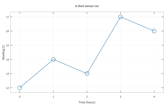
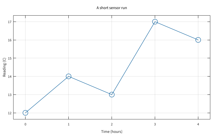
Plot the first measurements

A line and its markers show the order and values of a short run. Use padded axes so the endpoint markers remain fully visible.

Back to example overview

Compare with OCT-01-005 · Inspect the array shape.

Compare with gnuplot · First plot.

Complete Octave source

source ("config/plot-setup.m");
hours = 0:4;
readings = [12 14 13 17 16];
figure (1);
plot (hours, readings, "-o");
xlabel ("Time (hours)"); ylabel ("Reading (C)");
title ("A short sensor run"); grid on; axis padded;
print (gcf, "figures/OCT-01-006.pdf", "-dpdfcairo");
close all;
ParameterMeaning in this example
plot (hours, readings, "-o")Connect the five observations and mark each value.
axis paddedLeave room for the complete endpoint markers.
source / printUse the shared styling and native PDF export described above.

Run this example

tools/octave examples/OCT-01-006.m > examples/OCT-01-006.stdout.txt
python3 tools/pdf_metadata.py figures/OCT-01-006.pdf
pdftocairo -svg figures/OCT-01-006.pdf figures/OCT-01-006.svg
pdftocairo -png -singlefile -r 120 figures/OCT-01-006.pdf figures/OCT-01-006

Try changing: Change the reading at hour 3 from 17 to 15.

Actual plot

Plot the first measurements
OCT-01-006 · GNU Octave / gnuplot

GNU Octave · exit 0

Run this example
tools/octave examples/OCT-01-006.m > examples/OCT-01-006.stdout.txt
python3 tools/pdf_metadata.py figures/OCT-01-006.pdf
pdftocairo -svg figures/OCT-01-006.pdf figures/OCT-01-006.svg
pdftocairo -png -singlefile -r 120 figures/OCT-01-006.pdf figures/OCT-01-006

Download: Octave source · Source + local inputs ZIP · SVG plot · Native PDF · PNG preview

Try changing: Change the reading at hour 3 from 17 to 15.

02 · Matrices and indexing

Keep array orientation visible. Select by row, column or condition, then use the column-major ordering deliberately when reshaping a batch.

OCT-02-001

Transpose a sensor matrix

A transpose exchanges sensors and observation times. Use the dot transpose when you want to swap dimensions without conjugating complex values.

Back to example overview

Compare with OCT-01-004 · Arrange readings in a matrix.

Complete Octave source

readings = [11 12 13; 14 15 16];
disp (readings.');
ParameterMeaning in this example
.'Swap rows and columns without complex conjugation.

Run this example

tools/octave examples/OCT-02-001.m > examples/OCT-02-001.stdout.txt

Try changing: Add a third sensor row and inspect the transposed shape.

Actual numerical result

   11   14
   12   15
   13   16

GNU Octave · exit 0

Run this example
tools/octave examples/OCT-02-001.m > examples/OCT-02-001.stdout.txt

Download: Octave source · Source + local inputs ZIP · Captured output

Try changing: Add a third sensor row and inspect the transposed shape.

OCT-02-002

Select a row and a column

Two indices identify a value by row and column, starting at one. Use a colon to retain all entries along a selected dimension.

Back to example overview

Compare with OCT-02-001 · Transpose a sensor matrix.

Complete Octave source

readings = [11 12 13; 14 15 16];
printf ("Sensor 2, time 3: %d\n", readings(2, 3));
disp (readings(:, 2));
ParameterMeaning in this example
(2, 3)Select the third reading of the second sensor.
(:, 2)Keep all sensor rows at the second time.

Run this example

tools/octave examples/OCT-02-002.m > examples/OCT-02-002.stdout.txt

Try changing: Select the first sensor row instead of the second column.

Actual numerical result

Sensor 2, time 3: 16
   12
   15

GNU Octave · exit 0

Run this example
tools/octave examples/OCT-02-002.m > examples/OCT-02-002.stdout.txt

Download: Octave source · Source + local inputs ZIP · Captured output

Try changing: Select the first sensor row instead of the second column.

OCT-02-003

Inspect column-major order

One index walks through a matrix column by column. Use this ordering to understand which observation a flattened position refers to.

Back to example overview

Compare with OCT-02-002 · Select a row and a column.

Complete Octave source

readings = [11 12 13; 14 15 16];
printf ("Fourth linear element: %d\n", readings(4));
disp (readings(:).');
ParameterMeaning in this example
(4)Select the fourth element in column-major order.
(:)Flatten the full matrix into a column.

Run this example

tools/octave examples/OCT-02-003.m > examples/OCT-02-003.stdout.txt

Try changing: Predict the fifth linear element before printing it.

Actual numerical result

Fourth linear element: 15
   11   14   12   15   13   16

GNU Octave · exit 0

Run this example
tools/octave examples/OCT-02-003.m > examples/OCT-02-003.stdout.txt

Download: Octave source · Source + local inputs ZIP · Captured output

Try changing: Predict the fifth linear element before printing it.

OCT-02-004

Select readings by a condition

A logical mask selects only values that satisfy a test. Use it to express an acceptance rule without listing element positions.

Back to example overview

Compare with OCT-02-003 · Inspect column-major order.

Complete Octave source

readings = [9 12 15 7];
accepted = readings >= 10;
disp (accepted);
disp (readings(accepted));
ParameterMeaning in this example
>= 10Test every reading against the threshold.
(accepted)Select only the true mask positions.

Run this example

tools/octave examples/OCT-02-004.m > examples/OCT-02-004.stdout.txt

Try changing: Change the threshold to 13 and predict the selected values.

Actual numerical result

  0  1  1  0
   12   15

GNU Octave · exit 0

Run this example
tools/octave examples/OCT-02-004.m > examples/OCT-02-004.stdout.txt

Download: Octave source · Source + local inputs ZIP · Captured output

Try changing: Change the threshold to 13 and predict the selected values.

OCT-02-005

Replace flagged values in place

An indexed assignment changes only the rejected entries. Use NaN to keep their positions while marking the observations as missing.

Back to example overview

Compare with OCT-02-004 · Select readings by a condition.

Complete Octave source

readings = [9 12 15 7];
readings(readings < 10) = NaN;
disp (readings);
ParameterMeaning in this example
readings < 10Identify rejected positions.
= NaNReplace those entries while preserving array length.

Run this example

tools/octave examples/OCT-02-005.m > examples/OCT-02-005.stdout.txt

Try changing: Replace the flagged values with zero and explain why that changes later averages.

Actual numerical result

   NaN    12    15   NaN

GNU Octave · exit 0

Run this example
tools/octave examples/OCT-02-005.m > examples/OCT-02-005.stdout.txt

Download: Octave source · Source + local inputs ZIP · Captured output

Try changing: Replace the flagged values with zero and explain why that changes later averages.

OCT-02-006

Reshape a complete batch

Reshape changes the dimensions while preserving column-major element order. Use it when a device delivers a flat batch with a known number of sensors.

Back to example overview

Compare with OCT-02-005 · Replace flagged values in place.

Complete Octave source

batch = [11 14 12 15 13 16];
readings = reshape (batch, 2, 3);
disp (readings);
ParameterMeaning in this example
reshape (batch, 2, 3)Arrange six elements into two sensor rows and three time columns.

Run this example

tools/octave examples/OCT-02-006.m > examples/OCT-02-006.stdout.txt

Try changing: Reshape the same batch to three rows and two columns.

Actual numerical result

   11   12   13
   14   15   16

GNU Octave · exit 0

Run this example
tools/octave examples/OCT-02-006.m > examples/OCT-02-006.stdout.txt

Download: Octave source · Source + local inputs ZIP · Captured output

Try changing: Reshape the same batch to three rows and two columns.

03 · Array operations and data hygiene

Distinguish elementwise arithmetic from matrix algebra. Apply offsets, summarize dimensions and handle nonfinite values without losing the relationship between readings and their identifiers.

OCT-03-001

Square each measurement independently

Dot operators apply an operation to each entry. Use them when a vector represents independent measurements rather than a matrix transformation.

Back to example overview

Compare with OCT-02-001 · Transpose a sensor matrix.

Complete Octave source

readings = [2 3 4];
disp (readings .^ 2);
ParameterMeaning in this example
.^ 2Square each of the three entries separately.

Run this example

tools/octave examples/OCT-03-001.m > examples/OCT-03-001.stdout.txt

Try changing: Change the exponent to 3.

Actual numerical result

    4    9   16

GNU Octave · exit 0

Run this example
tools/octave examples/OCT-03-001.m > examples/OCT-03-001.stdout.txt

Download: Octave source · Source + local inputs ZIP · Captured output

Try changing: Change the exponent to 3.

OCT-03-002

Multiply two transformations

Matrix multiplication combines rows of the first matrix with columns of the second. Use it for a linear transformation, and compare its result with an elementwise product.

Back to example overview

Compare with OCT-03-001 · Square each measurement independently.

Complete Octave source

A = [2 1; 0 3];
B = [1 4; 2 1];
disp (A * B);
printf ("Elementwise comparison:\n");
disp (A .* B);
ParameterMeaning in this example
*Apply matrix multiplication.
.*Retain a visible elementwise baseline for the same inputs.

Run this example

tools/octave examples/OCT-03-002.m > examples/OCT-03-002.stdout.txt

Try changing: Change B(2,1) from 2 to 5 and predict which matrix-product entries change.

Actual numerical result

   4   9
   6   3
Elementwise comparison:
   2   4
   0   3

GNU Octave · exit 0

Run this example
tools/octave examples/OCT-03-002.m > examples/OCT-03-002.stdout.txt

Download: Octave source · Source + local inputs ZIP · Captured output

Try changing: Change B(2,1) from 2 to 5 and predict which matrix-product entries change.

OCT-03-003

Broadcast a column calibration

A row of offsets applies one correction per measurement column. Use compatible shapes to express the correction without manually repeating the offsets.

Back to example overview

Compare with OCT-03-002 · Multiply two transformations.

Complete Octave source

raw = [1 2; 3 4; 5 6];
offsets = [10 20];
corrected = raw + offsets;
disp (corrected);
ParameterMeaning in this example
raw + offsetsBroadcast the one-by-two offsets across three rows.

Run this example

tools/octave examples/OCT-03-003.m > examples/OCT-03-003.stdout.txt

Try changing: Change the offsets to [100 200].

Actual numerical result

   11   22
   13   24
   15   26

GNU Octave · exit 0

Run this example
tools/octave examples/OCT-03-003.m > examples/OCT-03-003.stdout.txt

Download: Octave source · Source + local inputs ZIP · Captured output

Try changing: Change the offsets to [100 200].

OCT-03-004

Reduce one dimension at a time

A reduction can summarize sensors or observation times. Use its dimension argument explicitly so an orientation change cannot silently change the question.

Back to example overview

Compare with OCT-03-003 · Broadcast a column calibration.

Complete Octave source

readings = [11 12 13; 14 15 16];
printf ("Column totals:\n"); disp (sum (readings, 1));
printf ("Row means:\n"); disp (mean (readings, 2));
ParameterMeaning in this example
sum (..., 1)Sum sensor rows within each time column.
mean (..., 2)Average time columns within each sensor row.

Run this example

tools/octave examples/OCT-03-004.m > examples/OCT-03-004.stdout.txt

Try changing: Swap the two dimension arguments and explain the resulting shapes.

Actual numerical result

Column totals:
   25   27   29
Row means:
   12
   15

GNU Octave · exit 0

Run this example
tools/octave examples/OCT-03-004.m > examples/OCT-03-004.stdout.txt

Download: Octave source · Source + local inputs ZIP · Captured output

Try changing: Swap the two dimension arguments and explain the resulting shapes.

OCT-03-005

Exclude nonfinite observations

NaN and infinity should not silently enter a finite-reading summary. Use isfinite to retain only observations that can contribute to this calculation.

Back to example overview

Compare with OCT-03-004 · Reduce one dimension at a time.

Complete Octave source

readings = [12 NaN 15 Inf 14];
valid = readings(isfinite (readings));
printf ("Finite observations: %d; mean: %.3f\n", ...
        numel (valid), mean (valid));
ParameterMeaning in this example
isfiniteReject both NaN and infinite entries.
numel (valid)Report how many observations remain.

Run this example

tools/octave examples/OCT-03-005.m > examples/OCT-03-005.stdout.txt

Try changing: Replace 14 with NaN and predict the count and mean.

Actual numerical result

Finite observations: 3; mean: 13.667

GNU Octave · exit 0

Run this example
tools/octave examples/OCT-03-005.m > examples/OCT-03-005.stdout.txt

Download: Octave source · Source + local inputs ZIP · Captured output

Try changing: Replace 14 with NaN and predict the count and mean.

OCT-03-006

Sort complete observation rows

A row sort keeps each measurement attached to its site identifier. Use multiple sort keys when a site contains several observation times.

Back to example overview

Compare with OCT-03-005 · Exclude nonfinite observations.

Complete Octave source

observations = [2 1 15; 1 2 13; 1 0 11; 2 0 14];
ordered = sortrows (observations, [1 2]);
disp (ordered);
ParameterMeaning in this example
[site hour reading]Treat each row as one complete observation.
sortrows (..., [1 2])Sort by site, then by hour within each site.

Run this example

tools/octave examples/OCT-03-006.m > examples/OCT-03-006.stdout.txt

Try changing: Reverse the secondary key with [1 -2].

Actual numerical result

    1    0   11
    1    2   13
    2    0   14
    2    1   15

GNU Octave · exit 0

Run this example
tools/octave examples/OCT-03-006.m > examples/OCT-03-006.stdout.txt

Download: Octave source · Source + local inputs ZIP · Captured output

Try changing: Reverse the secondary key with [1 -2].

04 · Text and data containers

Keep labels, heterogeneous fields and structured records explicit. Choose a character string, cell array or structure according to the information that must travel together.

OCT-04-001

Build a site label

Formatted text combines a stable identifier with a readable label. Use sprintf when the label should be stored for later output or annotation.

Back to example overview

Compare with OCT-01-005 · Inspect the array shape.

Complete Octave source

site = 3;
label = sprintf ("SITE-%02d", site);
printf ("Label: %s\n", label);
ParameterMeaning in this example
sprintfReturn the formatted text instead of printing it immediately.
%02dUse two digits with a leading zero.

Run this example

tools/octave examples/OCT-04-001.m > examples/OCT-04-001.stdout.txt

Try changing: Change site to 12 and the prefix to STATION.

Actual numerical result

Label: SITE-03

GNU Octave · exit 0

Run this example
tools/octave examples/OCT-04-001.m > examples/OCT-04-001.stdout.txt

Download: Octave source · Source + local inputs ZIP · Captured output

Try changing: Change site to 12 and the prefix to STATION.

OCT-04-002

Parse a reported number

A numeric-looking string must be converted before arithmetic. Use str2double for a report field, and inspect its NaN result for malformed text.

Back to example overview

Compare with OCT-04-001 · Build a site label.

Complete Octave source

reading = str2double ("14.25");
invalid = str2double ("missing");
printf ("Parsed: %.2f; invalid is NaN: %d\n", reading, isnan (invalid));
ParameterMeaning in this example
str2doubleConvert text to a numerical scalar.
isnanDetect the failed conversion explicitly.

Run this example

tools/octave examples/OCT-04-002.m > examples/OCT-04-002.stdout.txt

Try changing: Replace missing with 16.5 and inspect the second result.

Actual numerical result

Parsed: 14.25; invalid is NaN: 1

GNU Octave · exit 0

Run this example
tools/octave examples/OCT-04-002.m > examples/OCT-04-002.stdout.txt

Download: Octave source · Source + local inputs ZIP · Captured output

Try changing: Replace missing with 16.5 and inspect the second result.

OCT-04-003

Keep unlike fields in a cell array

A cell array can hold a label, a number and an array without forcing them into one numeric matrix. Use braces to retrieve the value inside a cell.

Back to example overview

Compare with OCT-04-002 · Parse a reported number.

Complete Octave source

sample = {"SITE-02", 14.5, [1 0 1]};
printf ("Site: %s; reading: %.1f\n", sample{1}, sample{2});
disp (sample{3});
ParameterMeaning in this example
{...}Store heterogeneous values in one cell array.
sample{3}Retrieve the third value rather than a one-cell container.

Run this example

tools/octave examples/OCT-04-003.m > examples/OCT-04-003.stdout.txt

Try changing: Change the third field to a four-entry quality mask.

Actual numerical result

Site: SITE-02; reading: 14.5
   1   0   1

GNU Octave · exit 0

Run this example
tools/octave examples/OCT-04-003.m > examples/OCT-04-003.stdout.txt

Download: Octave source · Source + local inputs ZIP · Captured output

Try changing: Change the third field to a four-entry quality mask.

OCT-04-004

Name the fields of a record

A structure gives each field an explicit name. Use it when a reader should not need to remember which numeric position holds the site or reading.

Back to example overview

Compare with OCT-04-003 · Keep unlike fields in a cell array.

Complete Octave source

sample = struct ("site", "SITE-02", "reading_C", 14.5);
printf ("%s: %.1f C\n", sample.site, sample.reading_C);
ParameterMeaning in this example
structConstruct the record with named fields.
.reading_CAccess the value and keep its unit visible in the field name.

Run this example

tools/octave examples/OCT-04-004.m > examples/OCT-04-004.stdout.txt

Try changing: Add a quality field and print it.

Actual numerical result

SITE-02: 14.5 C

GNU Octave · exit 0

Run this example
tools/octave examples/OCT-04-004.m > examples/OCT-04-004.stdout.txt

Download: Octave source · Source + local inputs ZIP · Captured output

Try changing: Add a quality field and print it.

OCT-04-005

Collect a structure array

A structure array keeps several records under the same field vocabulary. Use brackets around a numeric field list to collect values for calculation.

Back to example overview

Compare with OCT-04-004 · Name the fields of a record.

Complete Octave source

samples(1) = struct ("site", 1, "reading_C", 12);
samples(2) = struct ("site", 2, "reading_C", 15);
values = [samples.reading_C];
printf ("Records: %d; mean: %.2f C\n", numel (samples), mean (values));
ParameterMeaning in this example
samples(2)Store a second record with the same fields.
[samples.reading_C]Collect the numeric field values into one vector.

Run this example

tools/octave examples/OCT-04-005.m > examples/OCT-04-005.stdout.txt

Try changing: Add a third site with a reading of 18 C.

Actual numerical result

Records: 2; mean: 13.50 C

GNU Octave · exit 0

Run this example
tools/octave examples/OCT-04-005.m > examples/OCT-04-005.stdout.txt

Download: Octave source · Source + local inputs ZIP · Captured output

Try changing: Add a third site with a reading of 18 C.

OCT-04-006

Nest measurement metadata

Nested structures separate a measurement from its unit and collection metadata. Use dotted paths to make the record hierarchy visible.

Back to example overview

Compare with OCT-04-005 · Collect a structure array.

Complete Octave source

sample.measurement.value = 14.5;
sample.measurement.unit = "C";
sample.collection.site = "SITE-02";
printf ("%s: %.1f %s\n", sample.collection.site, ...
        sample.measurement.value, sample.measurement.unit);
ParameterMeaning in this example
.measurement.valueLocate the numeric value inside its measurement record.
.collection.siteKeep the collection identifier in a separate nested record.

Run this example

tools/octave examples/OCT-04-006.m > examples/OCT-04-006.stdout.txt

Try changing: Add collection.hour and print it beside the site.

Actual numerical result

SITE-02: 14.5 C

GNU Octave · exit 0

Run this example
tools/octave examples/OCT-04-006.m > examples/OCT-04-006.stdout.txt

Download: Octave source · Source + local inputs ZIP · Captured output

Try changing: Add collection.hour and print it beside the site.

05 · Functions and control flow

Name repeated calculations and make decisions visible. Bound loops, keep function inputs explicit and check the behavior that later analysis depends on.

OCT-05-001

Choose an acceptance outcome

An if statement chooses one output according to the quality condition. Use both branches so an out-of-range observation has an explicit outcome.

Back to example overview

Compare with OCT-02-004 · Select readings by a condition.

Complete Octave source

reading = 15;
if (reading >= 10 && reading <= 20)
  printf ("Accepted: %.1f C\n", reading);
else
  printf ("Held for review: %.1f C\n", reading);
endif
ParameterMeaning in this example
&&Require both scalar bounds to hold.
if / else / endifSelect exactly one reported outcome.

Run this example

tools/octave examples/OCT-05-001.m > examples/OCT-05-001.stdout.txt

Try changing: Change reading to 25 and inspect the alternative branch.

Actual numerical result

Accepted: 15.0 C

GNU Octave · exit 0

Run this example
tools/octave examples/OCT-05-001.m > examples/OCT-05-001.stdout.txt

Download: Octave source · Source + local inputs ZIP · Captured output

Try changing: Change reading to 25 and inspect the alternative branch.

OCT-05-002

Fill a preallocated result

A for loop applies the calibration to each observation in turn. Use a preallocated array when the final result size is already known.

Back to example overview

Compare with OCT-03-003 · Broadcast a column calibration.

Complete Octave source

voltage = [0.5 0.6 0.7 0.8];
temperature = zeros (size (voltage));
for k = 1:numel (voltage)
  temperature(k) = 20 * voltage(k) + 1;
endfor
disp (temperature);
ParameterMeaning in this example
zeros (size (...))Allocate the output with the same shape as the input.
for k = ...Visit each element once.

Run this example

tools/octave examples/OCT-05-002.m > examples/OCT-05-002.stdout.txt

Try changing: Replace the loop with 20 .* voltage + 1 and compare the result.

Actual numerical result

   11   13   15   17

GNU Octave · exit 0

Run this example
tools/octave examples/OCT-05-002.m > examples/OCT-05-002.stdout.txt

Download: Octave source · Source + local inputs ZIP · Captured output

Try changing: Replace the loop with 20 .* voltage + 1 and compare the result.

OCT-05-003

Bound a refinement loop

A while loop refines a value until it reaches the tolerance or the iteration limit. Use an explicit budget so an unexpected convergence problem cannot run forever.

Back to example overview

Compare with OCT-05-002 · Fill a preallocated result.

Complete Octave source

estimate = 0;
iterations = 0;
while (abs (estimate - 1) > 1e-3 && iterations < 10)
  estimate = (estimate + 1) / 2;
  iterations = iterations + 1;
endwhile
printf ("Iterations: %d; estimate: %.6f\n", iterations, estimate);
ParameterMeaning in this example
abs (...) > 1e-3Continue while the distance from the target is too large.
iterations < 10Limit the complete refinement to ten iterations.

Run this example

tools/octave examples/OCT-05-003.m > examples/OCT-05-003.stdout.txt

Try changing: Reduce the iteration budget to 4 and inspect the final error.

Actual numerical result

Iterations: 10; estimate: 0.999023

GNU Octave · exit 0

Run this example
tools/octave examples/OCT-05-003.m > examples/OCT-05-003.stdout.txt

Download: Octave source · Source + local inputs ZIP · Captured output

Try changing: Reduce the iteration budget to 4 and inspect the final error.

OCT-05-004

Name a small calculation with a handle

An anonymous function stores a short calculation with named inputs. Use elementwise operators so the same handle accepts a scalar or an array.

Back to example overview

Compare with OCT-05-003 · Bound a refinement loop.

Complete Octave source

calibrate = @(voltage) 20 .* voltage + 1;
disp (calibrate ([0.5 0.6 0.7]));
ParameterMeaning in this example
@(voltage)Create a function handle with one input.
calibrate (...)Call the stored calculation with a complete voltage vector.

Run this example

tools/octave examples/OCT-05-004.m > examples/OCT-05-004.stdout.txt

Try changing: Add a second argument for the offset.

Actual numerical result

   11   13   15

GNU Octave · exit 0

Run this example
tools/octave examples/OCT-05-004.m > examples/OCT-05-004.stdout.txt

Download: Octave source · Source + local inputs ZIP · Captured output

Try changing: Add a second argument for the offset.

OCT-05-005

Return two results from a local function

A local helper can return a minimum and a span together. Use this form when both values belong to the same calculation and should share one explicit input.

Back to example overview

Compare with OCT-05-004 · Name a small calculation with a handle.

Complete Octave source

1; % Mark this complete file as a script before its local helper.
function [lowest, span] = reading_limits (values)
  lowest = min (values);
  span = max (values) - lowest;
endfunction
[lowest, span] = reading_limits ([12 14 13 17]);
printf ("Minimum: %.1f C; span: %.1f C\n", lowest, span);
ParameterMeaning in this example
[lowest, span]Return and receive two values in a defined order.
1;Keep the file a script with its helper defined before use.

Run this example

tools/octave examples/OCT-05-005.m > examples/OCT-05-005.stdout.txt

Try changing: Return the maximum as a third output.

Actual numerical result

Minimum: 12.0 C; span: 5.0 C

GNU Octave · exit 0

Run this example
tools/octave examples/OCT-05-005.m > examples/OCT-05-005.stdout.txt

Download: Octave source · Source + local inputs ZIP · Captured output

Try changing: Return the maximum as a third output.

OCT-05-006

Check a calibration contract

An assertion makes the expected numerical behavior executable. Use a tolerance for floating-point values and retain a clear success message after the check.

Back to example overview

Compare with OCT-05-005 · Return two results from a local function.

Complete Octave source

calibrate = @(voltage) 20 .* voltage + 1;
actual = calibrate ([0.5 0.6 0.7]);
assert (actual, [11 13 15], 1e-10);
printf ("Three calibration checks passed.\n");
ParameterMeaning in this example
assert (actual, expected, tolerance)Require all three values to match within 1e-10.
Success messagePrint only after the check has passed.

Run this example

tools/octave examples/OCT-05-006.m > examples/OCT-05-006.stdout.txt

Try changing: Change the gain to 21 and observe the failed contract.

Actual numerical result

Three calibration checks passed.

GNU Octave · exit 0

Run this example
tools/octave examples/OCT-05-006.m > examples/OCT-05-006.stdout.txt

Download: Octave source · Source + local inputs ZIP · Captured output

Try changing: Change the gain to 21 and observe the failed contract.

06 · Scientific plotting fundamentals

Choose a visual form that matches the numerical question. Keep units, scales, legends and uncertainty explicit; the shared setup supplies the same page, font and palette for every plot.

OCT-06-001

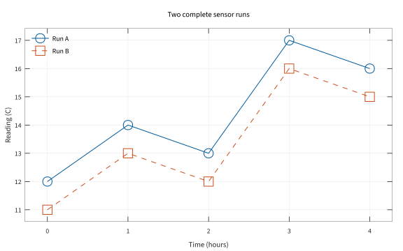
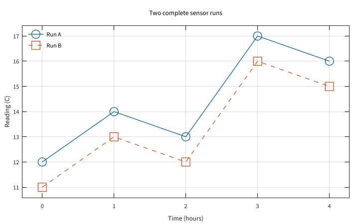
Compare two sensor runs

Two series on the same axes make their level difference visible. Use a legend with concrete run names and a location that leaves the observations unobscured.

Back to example overview

Compare with OCT-01-006 · Plot the first measurements.

Complete Octave source

source ("config/plot-setup.m");
hours = 0:4;
run_a = [12 14 13 17 16]; run_b = [11 13 12 16 15];
figure (1); plot (hours, run_a, "-o", hours, run_b, "--s");
xlabel ("Time (hours)"); ylabel ("Reading (C)");
key = legend ("Run A", "Run B", "location", "northwest");
set (key, "fontsize", 11, "box", "off");
title ("Two complete sensor runs"); grid on; axis padded;
print (gcf, "figures/OCT-06-001.pdf", "-dpdfcairo");
close all;
ParameterMeaning in this example
Two x/y pairsPlot both complete runs on shared axes.
legendIdentify each series by name.

Run this example

tools/octave examples/OCT-06-001.m > examples/OCT-06-001.stdout.txt
python3 tools/pdf_metadata.py figures/OCT-06-001.pdf
pdftocairo -svg figures/OCT-06-001.pdf figures/OCT-06-001.svg
pdftocairo -png -singlefile -r 120 figures/OCT-06-001.pdf figures/OCT-06-001

Try changing: Increase only Run B by 1 C and compare the gap.

Actual plot

Compare two sensor runs
OCT-06-001 · GNU Octave / gnuplot

GNU Octave · exit 0

Run this example
tools/octave examples/OCT-06-001.m > examples/OCT-06-001.stdout.txt
python3 tools/pdf_metadata.py figures/OCT-06-001.pdf
pdftocairo -svg figures/OCT-06-001.pdf figures/OCT-06-001.svg
pdftocairo -png -singlefile -r 120 figures/OCT-06-001.pdf figures/OCT-06-001

Download: Octave source · Source + local inputs ZIP · SVG plot · Native PDF · PNG preview

Try changing: Increase only Run B by 1 C and compare the gap.

OCT-06-002

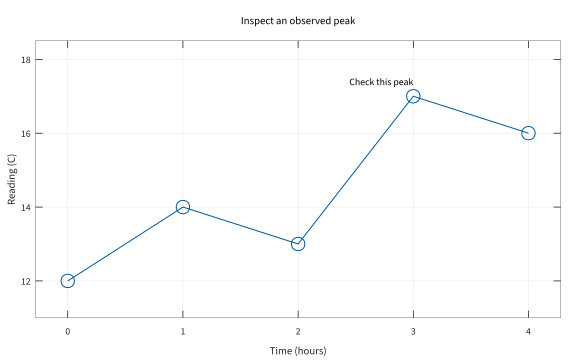
Annotate a reading of interest

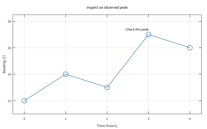
A text annotation explains why one observed point deserves attention. Use data coordinates and reserve vertical room for the label.

Back to example overview

Compare with OCT-01-006 · Plot the first measurements.

Complete Octave source

source ("config/plot-setup.m");
hours = 0:4; readings = [12 14 13 17 16];
figure (1); plot (hours, readings, "-o");
xlabel ("Time (hours)"); ylabel ("Reading (C)");
title ("Inspect an observed peak"); grid on; axis padded;
ylim ([11 18.5]);
text (3, 17.4, "Check this peak", "horizontalalignment", "right");
print (gcf, "figures/OCT-06-002.pdf", "-dpdfcairo");
close all;
ParameterMeaning in this example
text (3, 17.4, ...)Anchor the note above the peak at hour 3.
ylimKeep the annotation inside the exported axes.

Run this example

tools/octave examples/OCT-06-002.m > examples/OCT-06-002.stdout.txt
python3 tools/pdf_metadata.py figures/OCT-06-002.pdf
pdftocairo -svg figures/OCT-06-002.pdf figures/OCT-06-002.svg
pdftocairo -png -singlefile -r 120 figures/OCT-06-002.pdf figures/OCT-06-002

Try changing: Move the note to the reading at hour 1 and revise its wording.

Actual plot

Annotate a reading of interest
OCT-06-002 · GNU Octave / gnuplot

GNU Octave · exit 0

Run this example
tools/octave examples/OCT-06-002.m > examples/OCT-06-002.stdout.txt
python3 tools/pdf_metadata.py figures/OCT-06-002.pdf
pdftocairo -svg figures/OCT-06-002.pdf figures/OCT-06-002.svg
pdftocairo -png -singlefile -r 120 figures/OCT-06-002.pdf figures/OCT-06-002

Download: Octave source · Source + local inputs ZIP · SVG plot · Native PDF · PNG preview

Try changing: Move the note to the reading at hour 1 and revise its wording.

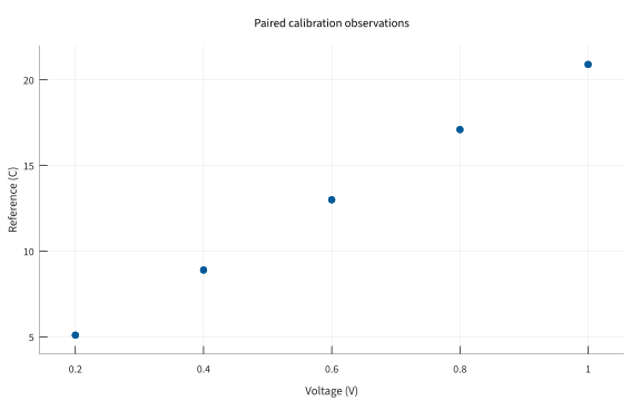
OCT-06-003

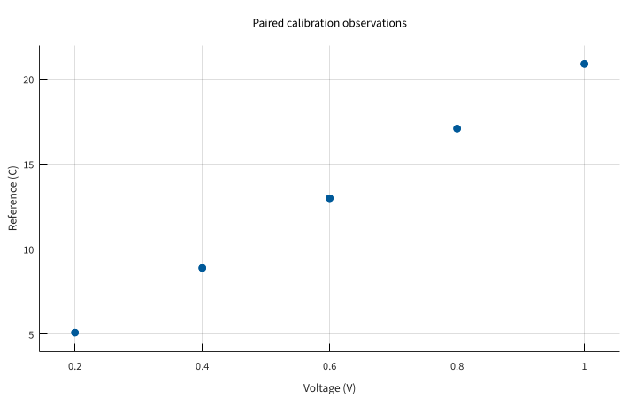
Inspect a pairwise relationship

A scatter plot shows paired observations without implying an ordering between neighboring markers. Use it when a voltage and its reference temperature belong to the same sample.

Back to example overview

Compare with OCT-01-006 · Plot the first measurements.

Complete Octave source

source ("config/plot-setup.m");
voltage = [0.2 0.4 0.6 0.8 1.0];
reference = [5.1 8.9 13.0 17.1 20.9];
figure (1); scatter (voltage, reference, 45, "filled");
xlabel ("Voltage (V)"); ylabel ("Reference (C)");
title ("Paired calibration observations"); grid on; axis padded;
print (gcf, "figures/OCT-06-003.pdf", "-dpdfcairo");
close all;
ParameterMeaning in this example
scatterRepresent each voltage/reference pair with one marker.
45Choose a common marker area in points squared.

Run this example

tools/octave examples/OCT-06-003.m > examples/OCT-06-003.stdout.txt
python3 tools/pdf_metadata.py figures/OCT-06-003.pdf
pdftocairo -svg figures/OCT-06-003.pdf figures/OCT-06-003.svg
pdftocairo -png -singlefile -r 120 figures/OCT-06-003.pdf figures/OCT-06-003

Try changing: Change one reference value and identify its point on the plot.

Actual plot

Inspect a pairwise relationship
OCT-06-003 · GNU Octave / gnuplot

GNU Octave · exit 0

Run this example
tools/octave examples/OCT-06-003.m > examples/OCT-06-003.stdout.txt
python3 tools/pdf_metadata.py figures/OCT-06-003.pdf
pdftocairo -svg figures/OCT-06-003.pdf figures/OCT-06-003.svg
pdftocairo -png -singlefile -r 120 figures/OCT-06-003.pdf figures/OCT-06-003

Download: Octave source · Source + local inputs ZIP · SVG plot · Native PDF · PNG preview

Try changing: Change one reference value and identify its point on the plot.

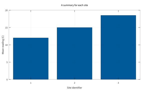
OCT-06-004

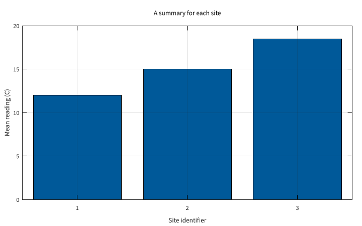
Compare site summaries with bars

Bars compare the three site means on a common baseline. Use explicit site ticks so interpolated numerical positions are not mistaken for additional sites.

Back to example overview

Compare with OCT-06-003 · Inspect a pairwise relationship.

Complete Octave source

source ("config/plot-setup.m");
sites = 1:3; site_mean = [12 15 18.5];
figure (1); bar (sites, site_mean);
set (gca, "xtick", sites);
xlabel ("Site identifier"); ylabel ("Mean reading (C)");
title ("A summary for each site"); grid on;
print (gcf, "figures/OCT-06-004.pdf", "-dpdfcairo");
close all;
ParameterMeaning in this example
barCompare three named site positions.
xtickDisplay only the actual integer site identifiers.

Run this example

tools/octave examples/OCT-06-004.m > examples/OCT-06-004.stdout.txt
python3 tools/pdf_metadata.py figures/OCT-06-004.pdf
pdftocairo -svg figures/OCT-06-004.pdf figures/OCT-06-004.svg
pdftocairo -png -singlefile -r 120 figures/OCT-06-004.pdf figures/OCT-06-004

Try changing: Change the third site mean to 17 C.

Actual plot

Compare site summaries with bars
OCT-06-004 · GNU Octave / gnuplot

GNU Octave · exit 0

Run this example
tools/octave examples/OCT-06-004.m > examples/OCT-06-004.stdout.txt
python3 tools/pdf_metadata.py figures/OCT-06-004.pdf
pdftocairo -svg figures/OCT-06-004.pdf figures/OCT-06-004.svg
pdftocairo -png -singlefile -r 120 figures/OCT-06-004.pdf figures/OCT-06-004

Download: Octave source · Source + local inputs ZIP · SVG plot · Native PDF · PNG preview

Try changing: Change the third site mean to 17 C.

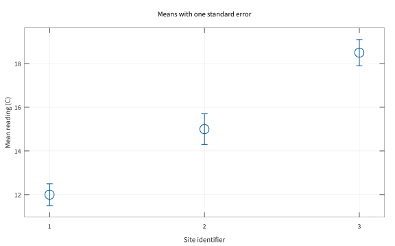
OCT-06-005

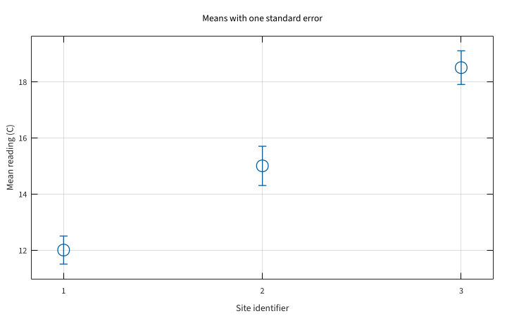
State the meaning of error bars

The supplied errors are illustrative one-standard-error values for the three means. Use an uncertainty label and units so the reader does not have to guess what the bars represent.

Back to example overview

Compare with OCT-06-004 · Compare site summaries with bars.

Complete Octave source

source ("config/plot-setup.m");
sites = 1:3; site_mean = [12 15 18.5];
standard_error = [0.5 0.7 0.6];
figure (1); errorbar (sites, site_mean, standard_error, "o");
set (gca, "xtick", sites);
xlabel ("Site identifier"); ylabel ("Mean reading (C)");
title ("Means with one standard error"); grid on; axis padded;
print (gcf, "figures/OCT-06-005.pdf", "-dpdfcairo");
close all;
ParameterMeaning in this example
errorbarDraw the supplied symmetric standard errors.
standard_errorUse errors in the same C unit as the means.

Run this example

tools/octave examples/OCT-06-005.m > examples/OCT-06-005.stdout.txt
python3 tools/pdf_metadata.py figures/OCT-06-005.pdf
pdftocairo -svg figures/OCT-06-005.pdf figures/OCT-06-005.svg
pdftocairo -png -singlefile -r 120 figures/OCT-06-005.pdf figures/OCT-06-005

Try changing: Double the standard errors while keeping the means fixed.

Actual plot

State the meaning of error bars
OCT-06-005 · GNU Octave / gnuplot

GNU Octave · exit 0

Run this example
tools/octave examples/OCT-06-005.m > examples/OCT-06-005.stdout.txt
python3 tools/pdf_metadata.py figures/OCT-06-005.pdf
pdftocairo -svg figures/OCT-06-005.pdf figures/OCT-06-005.svg
pdftocairo -png -singlefile -r 120 figures/OCT-06-005.pdf figures/OCT-06-005

Download: Octave source · Source + local inputs ZIP · SVG plot · Native PDF · PNG preview

Try changing: Double the standard errors while keeping the means fixed.

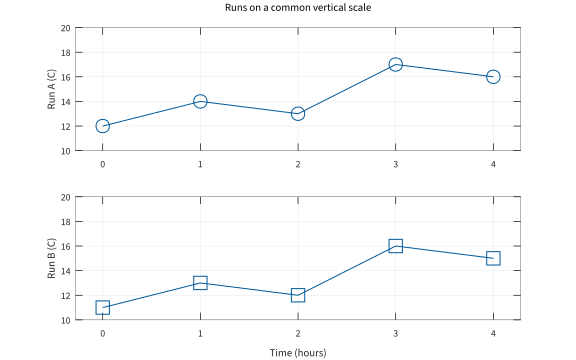
OCT-06-006

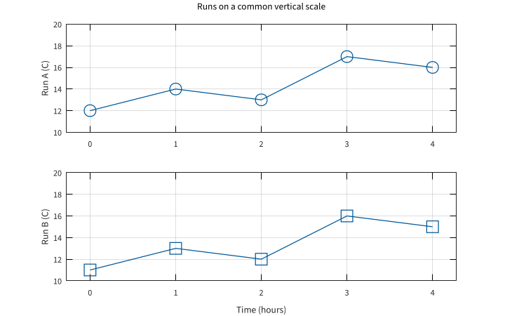
Align two panels on a common scale

Separate panels make each run readable while preserving a fair comparison. Use the same vertical limits so a small change in one panel is not visually exaggerated.

Back to example overview

Compare with OCT-06-001 · Compare two sensor runs.

Complete Octave source

source ("config/plot-setup.m");
hours = 0:4; run_a = [12 14 13 17 16]; run_b = [11 13 12 16 15];
figure (1);
subplot (2, 1, 1); plot (hours, run_a, "-o");
ylabel ("Run A (C)"); title ("Runs on a common vertical scale");
grid on; axis padded; ylim ([10 20]);
subplot (2, 1, 2); plot (hours, run_b, "-s");
xlabel ("Time (hours)"); ylabel ("Run B (C)");
grid on; axis padded; ylim ([10 20]);
print (gcf, "figures/OCT-06-006.pdf", "-dpdfcairo");
close all;
ParameterMeaning in this example
subplot (2, 1, n)Select one of two vertically stacked panels.
ylim ([10 20])Give both panels the same vertical range.

Run this example

tools/octave examples/OCT-06-006.m > examples/OCT-06-006.stdout.txt
python3 tools/pdf_metadata.py figures/OCT-06-006.pdf
pdftocairo -svg figures/OCT-06-006.pdf figures/OCT-06-006.svg
pdftocairo -png -singlefile -r 120 figures/OCT-06-006.pdf figures/OCT-06-006

Try changing: Change only Run B and confirm that both vertical scales remain identical.

Actual plot

Align two panels on a common scale
OCT-06-006 · GNU Octave / gnuplot

GNU Octave · exit 0

Run this example
tools/octave examples/OCT-06-006.m > examples/OCT-06-006.stdout.txt
python3 tools/pdf_metadata.py figures/OCT-06-006.pdf
pdftocairo -svg figures/OCT-06-006.pdf figures/OCT-06-006.svg
pdftocairo -png -singlefile -r 120 figures/OCT-06-006.pdf figures/OCT-06-006

Download: Octave source · Source + local inputs ZIP · SVG plot · Native PDF · PNG preview

Try changing: Change only Run B and confirm that both vertical scales remain identical.

07 · Distributions, fields and surfaces

Select a scale or geometry that reveals the structure in the data. All fields here are small, synthetic and generated locally; no remote map, image or dataset is needed.

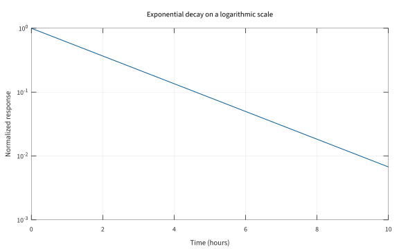
OCT-07-001

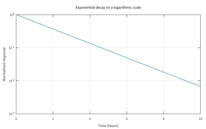
Inspect exponential decay on a log scale

A logarithmic vertical scale turns this exponential decay into a straight trend. Use it for positive values spanning several orders of magnitude.

Back to example overview

Compare with OCT-01-006 · Plot the first measurements.

Complete Octave source

source ("config/plot-setup.m");
hours = linspace (0, 10, 101);
response = exp (-0.5 .* hours);
figure (1); semilogy (hours, response);
xlabel ("Time (hours)"); ylabel ("Normalized response");
title ("Exponential decay on a logarithmic scale"); grid on;
print (gcf, "figures/OCT-07-001.pdf", "-dpdfcairo");
close all;
ParameterMeaning in this example
semilogyUse logarithmic y coordinates and linear time.
exp (-0.5 .* hours)Generate the synthetic positive decay.

Run this example

tools/octave examples/OCT-07-001.m > examples/OCT-07-001.stdout.txt
python3 tools/pdf_metadata.py figures/OCT-07-001.pdf
pdftocairo -svg figures/OCT-07-001.pdf figures/OCT-07-001.svg
pdftocairo -png -singlefile -r 120 figures/OCT-07-001.pdf figures/OCT-07-001

Try changing: Change the decay coefficient to 0.8.

Actual plot

Inspect exponential decay on a log scale
OCT-07-001 · GNU Octave / gnuplot

GNU Octave · exit 0

Run this example
tools/octave examples/OCT-07-001.m > examples/OCT-07-001.stdout.txt
python3 tools/pdf_metadata.py figures/OCT-07-001.pdf
pdftocairo -svg figures/OCT-07-001.pdf figures/OCT-07-001.svg
pdftocairo -png -singlefile -r 120 figures/OCT-07-001.pdf figures/OCT-07-001

Download: Octave source · Source + local inputs ZIP · SVG plot · Native PDF · PNG preview

Try changing: Change the decay coefficient to 0.8.

OCT-07-002

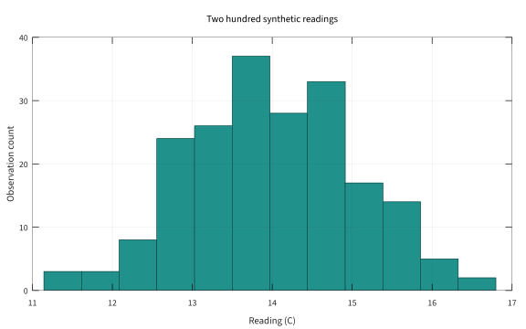
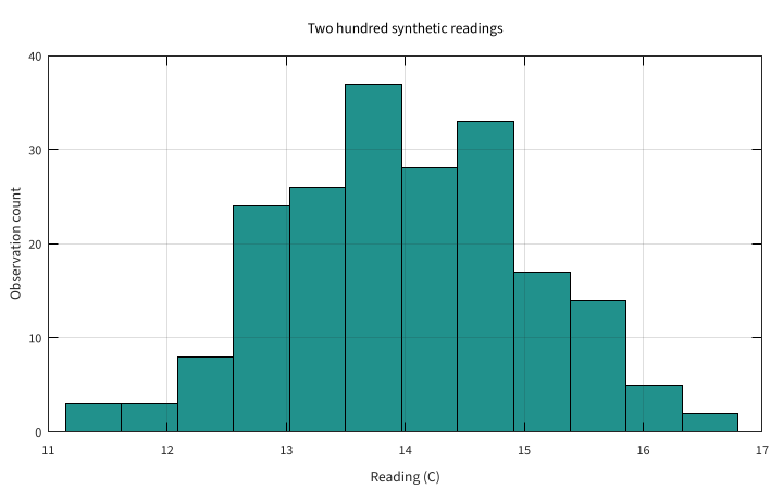
Show a repeatable distribution

A histogram summarizes the shape of repeated synthetic readings. Use a stated seed so changes in the bin count can be compared against the same observations.

Back to example overview

Compare with OCT-07-001 · Inspect exponential decay on a log scale.

Complete Octave source

source ("config/plot-setup.m");
rng (17, "twister");
readings = 14 + randn (1, 200);
figure (1); hist (readings, 12);
xlabel ("Reading (C)"); ylabel ("Observation count");
title ("Two hundred synthetic readings"); grid on;
print (gcf, "figures/OCT-07-002.pdf", "-dpdfcairo");
close all;
ParameterMeaning in this example
rng (17, "twister")Fix the random generator before drawing observations.
hist (..., 12)Summarize the same sample with twelve bins.

Run this example

tools/octave examples/OCT-07-002.m > examples/OCT-07-002.stdout.txt
python3 tools/pdf_metadata.py figures/OCT-07-002.pdf
pdftocairo -svg figures/OCT-07-002.pdf figures/OCT-07-002.svg
pdftocairo -png -singlefile -r 120 figures/OCT-07-002.pdf figures/OCT-07-002

Try changing: Use six bins without changing the seed.

Actual plot

Show a repeatable distribution
OCT-07-002 · GNU Octave / gnuplot

GNU Octave · exit 0

Run this example
tools/octave examples/OCT-07-002.m > examples/OCT-07-002.stdout.txt
python3 tools/pdf_metadata.py figures/OCT-07-002.pdf
pdftocairo -svg figures/OCT-07-002.pdf figures/OCT-07-002.svg
pdftocairo -png -singlefile -r 120 figures/OCT-07-002.pdf figures/OCT-07-002

Download: Octave source · Source + local inputs ZIP · SVG plot · Native PDF · PNG preview

Try changing: Use six bins without changing the seed.

OCT-07-003

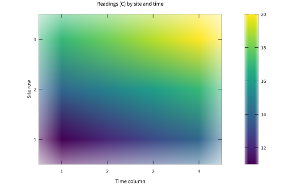
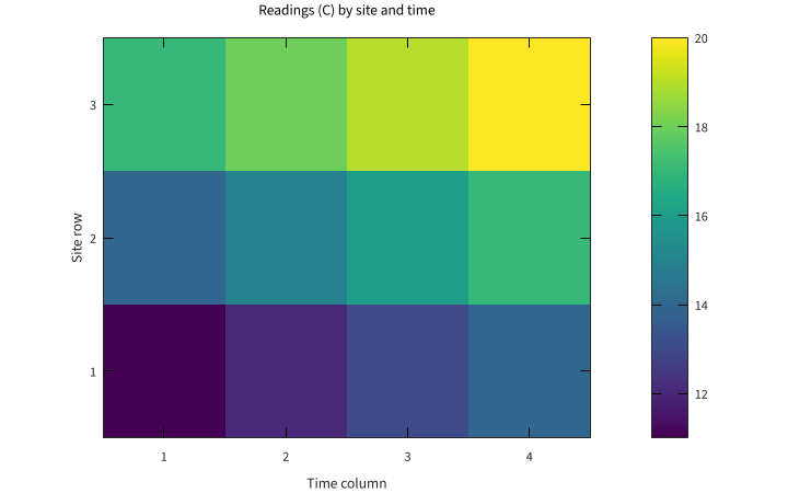
Map a measurement matrix to color

Each colored cell represents one site/time entry. Use an explicit orientation and ticks so the color grid preserves the matrix meaning.

Back to example overview

Compare with OCT-07-002 · Show a repeatable distribution.

Complete Octave source

source ("config/plot-setup.m");
readings = [11 12 13 14; 14 15 16 17; 17 18 19 20];
figure (1); imagesc (readings); axis xy;
set (gca, "xtick", 1:4, "ytick", 1:3);
colormap (viridis (128)); colorbar;
xlabel ("Time column"); ylabel ("Site row");
title ("Readings (C) by site and time");
print (gcf, "figures/OCT-07-003.pdf", "-dpdfcairo");
close all;
ParameterMeaning in this example
imagescMap the numerical matrix range into colors.
axis xyPlace smaller site indices lower on the vertical axis.
viridis / colorbarUse one ordered palette and show its numerical range.

Run this example

tools/octave examples/OCT-07-003.m > examples/OCT-07-003.stdout.txt
python3 tools/pdf_metadata.py figures/OCT-07-003.pdf
pdftocairo -svg figures/OCT-07-003.pdf figures/OCT-07-003.svg
pdftocairo -png -singlefile -r 120 figures/OCT-07-003.pdf figures/OCT-07-003

Try changing: Raise the middle row by 2 C and inspect the color range.

Actual plot

Map a measurement matrix to color
OCT-07-003 · GNU Octave / gnuplot

GNU Octave · exit 0

Run this example
tools/octave examples/OCT-07-003.m > examples/OCT-07-003.stdout.txt
python3 tools/pdf_metadata.py figures/OCT-07-003.pdf
pdftocairo -svg figures/OCT-07-003.pdf figures/OCT-07-003.svg
pdftocairo -png -singlefile -r 120 figures/OCT-07-003.pdf figures/OCT-07-003

Download: Octave source · Source + local inputs ZIP · SVG plot · Native PDF · PNG preview

Try changing: Raise the middle row by 2 C and inspect the color range.

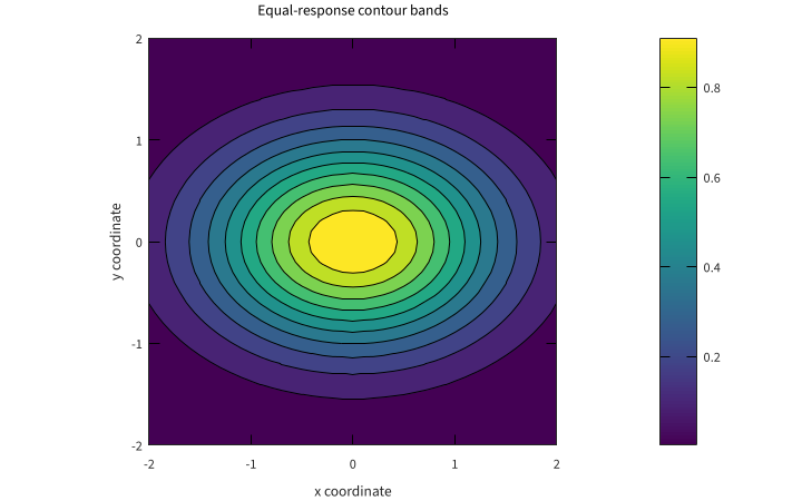
OCT-07-004

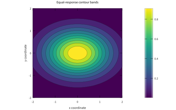
Read a smooth field as contours

Contour bands summarize levels of one synthetic response field. Use this view when the location of equal values matters more than a three-dimensional projection.

Back to example overview

Compare with OCT-07-003 · Map a measurement matrix to color.

Complete Octave source

source ("config/plot-setup.m");
[x, y] = meshgrid (linspace (-2, 2, 41));
response = exp (-0.5 .* (x.^2 + 2 .* y.^2));
figure (1); contourf (x, y, response, 10);
axis equal tight; colormap (viridis (128)); colorbar;
xlabel ("x coordinate"); ylabel ("y coordinate");
title ("Equal-response contour bands");
print (gcf, "figures/OCT-07-004.pdf", "-dpdfcairo");
close all;
ParameterMeaning in this example
meshgridGenerate coordinate arrays for the full field.
contourf (..., 10)Draw ten filled response levels.

Run this example

tools/octave examples/OCT-07-004.m > examples/OCT-07-004.stdout.txt
python3 tools/pdf_metadata.py figures/OCT-07-004.pdf
pdftocairo -svg figures/OCT-07-004.pdf figures/OCT-07-004.svg
pdftocairo -png -singlefile -r 120 figures/OCT-07-004.pdf figures/OCT-07-004

Try changing: Change the coefficient of y squared from 2 to 0.5.

Actual plot

Read a smooth field as contours
OCT-07-004 · GNU Octave / gnuplot

GNU Octave · exit 0

Run this example
tools/octave examples/OCT-07-004.m > examples/OCT-07-004.stdout.txt
python3 tools/pdf_metadata.py figures/OCT-07-004.pdf
pdftocairo -svg figures/OCT-07-004.pdf figures/OCT-07-004.svg
pdftocairo -png -singlefile -r 120 figures/OCT-07-004.pdf figures/OCT-07-004

Download: Octave source · Source + local inputs ZIP · SVG plot · Native PDF · PNG preview

Try changing: Change the coefficient of y squared from 2 to 0.5.

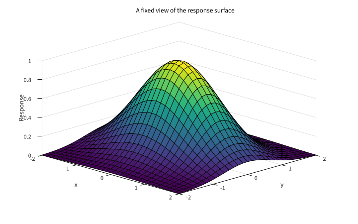
OCT-07-005

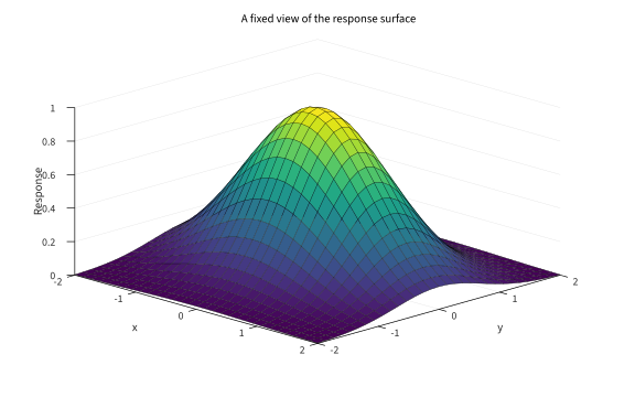
Inspect the same field as a surface

A fixed three-dimensional view exposes the response height directly. Use a fixed camera so two renders can be compared without viewpoint changes.

Back to example overview

Compare with OCT-07-004 · Read a smooth field as contours.

Complete Octave source

source ("config/plot-setup.m");
[x, y] = meshgrid (linspace (-2, 2, 31));
response = exp (-0.5 .* (x.^2 + 2 .* y.^2));
figure (1); surf (x, y, response);
view (45, 30); colormap (viridis (128));
xlabel ("x"); ylabel ("y"); zlabel ("Response");
title ("A fixed view of the response surface");
print (gcf, "figures/OCT-07-005.pdf", "-dpdfcairo");
close all;
ParameterMeaning in this example
surfDraw field values as surface heights.
view (45, 30)Fix azimuth and elevation in degrees.

Run this example

tools/octave examples/OCT-07-005.m > examples/OCT-07-005.stdout.txt
python3 tools/pdf_metadata.py figures/OCT-07-005.pdf
pdftocairo -svg figures/OCT-07-005.pdf figures/OCT-07-005.svg
pdftocairo -png -singlefile -r 120 figures/OCT-07-005.pdf figures/OCT-07-005

Try changing: Change only the view to 60 degrees azimuth and keep the field fixed.

Actual plot

Inspect the same field as a surface
OCT-07-005 · GNU Octave / gnuplot

GNU Octave · exit 0

Native diagnostics
multiplot> set style increment default;
                               ^
           line 0: warning: deprecated command
Run this example
tools/octave examples/OCT-07-005.m > examples/OCT-07-005.stdout.txt
python3 tools/pdf_metadata.py figures/OCT-07-005.pdf
pdftocairo -svg figures/OCT-07-005.pdf figures/OCT-07-005.svg
pdftocairo -png -singlefile -r 120 figures/OCT-07-005.pdf figures/OCT-07-005

Download: Octave source · Source + local inputs ZIP · SVG plot · Native PDF · PNG preview

Try changing: Change only the view to 60 degrees azimuth and keep the field fixed.

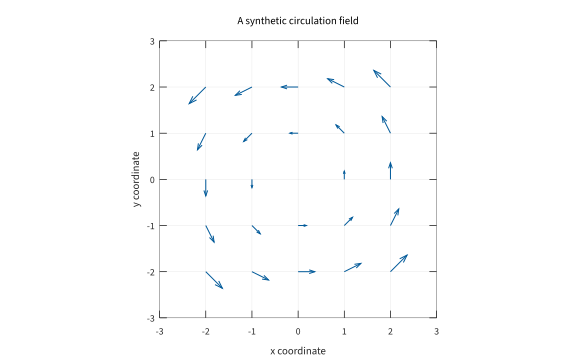
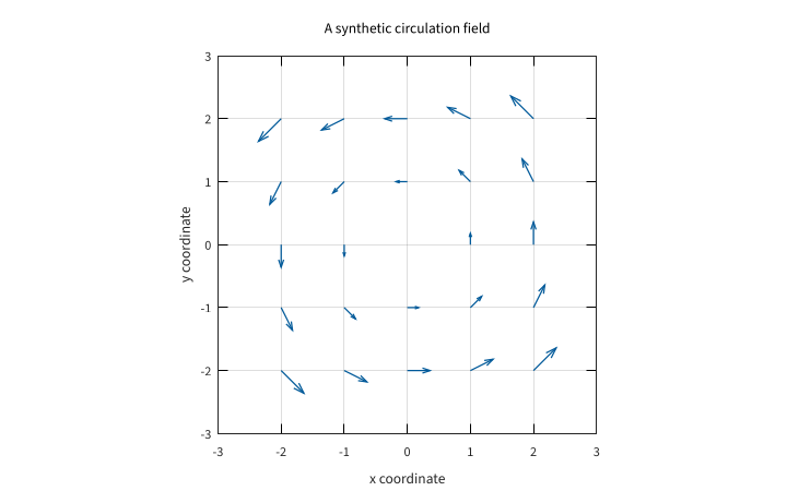
OCT-07-006

Show direction with a vector field

Arrow direction and length represent a synthetic circulation field. Use equal coordinate scales and enough space for complete arrowheads.

Back to example overview

Compare with OCT-07-005 · Inspect the same field as a surface.

Complete Octave source

source ("config/plot-setup.m");
[x, y] = meshgrid (-2:1:2);
u = -y; v = x;
figure (1); quiver (x, y, u, v, 0.45);
axis ([-3 3 -3 3]); axis equal;
xlabel ("x coordinate"); ylabel ("y coordinate");
title ("A synthetic circulation field"); grid on;
print (gcf, "figures/OCT-07-006.pdf", "-dpdfcairo");
close all;
ParameterMeaning in this example
quiverDraw one vector from each grid point.
0.45Reduce arrow scaling to separate neighboring arrows.
[-3 3 -3 3]Retain the full arrowheads inside fixed limits.

Run this example

tools/octave examples/OCT-07-006.m > examples/OCT-07-006.stdout.txt
python3 tools/pdf_metadata.py figures/OCT-07-006.pdf
pdftocairo -svg figures/OCT-07-006.pdf figures/OCT-07-006.svg
pdftocairo -png -singlefile -r 120 figures/OCT-07-006.pdf figures/OCT-07-006

Try changing: Reverse both components to reverse the circulation.

Actual plot

Show direction with a vector field
OCT-07-006 · GNU Octave / gnuplot

GNU Octave · exit 0

Run this example
tools/octave examples/OCT-07-006.m > examples/OCT-07-006.stdout.txt
python3 tools/pdf_metadata.py figures/OCT-07-006.pdf
pdftocairo -svg figures/OCT-07-006.pdf figures/OCT-07-006.svg
pdftocairo -png -singlefile -r 120 figures/OCT-07-006.pdf figures/OCT-07-006

Download: Octave source · Source + local inputs ZIP · SVG plot · Native PDF · PNG preview

Try changing: Reverse both components to reverse the circulation.

08 · Linear algebra and numerical reliability

Solve the stated system and inspect the quality of the result. Distinguish an exact solve, a least-squares fit and a low-rank approximation, and keep conditioning separate from residual size.

OCT-08-001

Solve a linear system directly

Left division solves the two coupled equations without explicitly forming an inverse. Use a residual to check that the computed solution satisfies the original system.

Back to example overview

Compare with OCT-03-002 · Multiply two transformations.

Complete Octave source

A = [2 1; 1 3]; b = [5; 7];
x = A \ b;
printf ("Solution: %.6f %.6f\n", x(1), x(2));
printf ("Residual norm: %.9f\n", norm (A * x - b));
ParameterMeaning in this example
A \ bSolve the complete system for x.
norm (A*x-b)Check the residual in the original equations.

Run this example

tools/octave examples/OCT-08-001.m > examples/OCT-08-001.stdout.txt

Try changing: Change b to [6; 8] and inspect the new residual.

Actual numerical result

Solution: 1.600000 1.800000
Residual norm: 0.000000000

GNU Octave · exit 0

Run this example
tools/octave examples/OCT-08-001.m > examples/OCT-08-001.stdout.txt

Download: Octave source · Source + local inputs ZIP · Captured output

Try changing: Change b to [6; 8] and inspect the new residual.

OCT-08-002

Fit an overdetermined linear model

More observations than coefficients lead to a least-squares problem. Use a design matrix with an intercept column to state the model explicitly.

Back to example overview

Compare with OCT-08-001 · Solve a linear system directly.

Complete Octave source

hours = (0:3).'; readings = [11; 12; 13; 14];
A = [ones(4, 1), hours];
coefficients = A \ readings;
printf ("Intercept: %.6f C; slope: %.6f C/hour\n", ...
        coefficients(1), coefficients(2));
ParameterMeaning in this example
[ones(...), hours]Specify intercept and time as separate model columns.
A \ readingsCompute the least-squares coefficients.

Run this example

tools/octave examples/OCT-08-002.m > examples/OCT-08-002.stdout.txt

Try changing: Raise only the final observation by 1 C.

Actual numerical result

Intercept: 11.000000 C; slope: 1.000000 C/hour

GNU Octave · exit 0

Run this example
tools/octave examples/OCT-08-002.m > examples/OCT-08-002.stdout.txt

Download: Octave source · Source + local inputs ZIP · Captured output

Try changing: Raise only the final observation by 1 C.

OCT-08-003

Check the eigenmodes of a symmetric matrix

Eigenvalues describe the action of this symmetric two-state transformation. Use the decomposition residual to verify the returned modes without relying on arbitrary vector signs.

Back to example overview

Compare with OCT-08-002 · Fit an overdetermined linear model.

Complete Octave source

A = [2 -1; -1 2];
[V, D] = eig (A);
printf ("Eigenvalues: %.6f %.6f\n", sort (diag (D)));
printf ("Mode residual: %.9f\n", norm (A * V - V * D));
ParameterMeaning in this example
eigReturn eigenvectors and their diagonal eigenvalue matrix.
A*V-V*DCheck the defining relation for every mode.

Run this example

tools/octave examples/OCT-08-003.m > examples/OCT-08-003.stdout.txt

Try changing: Change the two diagonal entries from 2 to 3.

Actual numerical result

Eigenvalues: 1.000000 3.000000
Mode residual: 0.000000000

GNU Octave · exit 0

Run this example
tools/octave examples/OCT-08-003.m > examples/OCT-08-003.stdout.txt

Download: Octave source · Source + local inputs ZIP · Captured output

Try changing: Change the two diagonal entries from 2 to 3.

OCT-08-004

Retain one singular component

A truncated singular-value decomposition approximates the matrix with one component. Use its reconstruction error to quantify what the compression removes.

Back to example overview

Compare with OCT-08-003 · Check the eigenmodes of a symmetric matrix.

Complete Octave source

A = [1 2 3; 2 4 6; 1 3 4];
[U, S, V] = svd (A);
rank_one = U(:, 1) * S(1, 1) * V(:, 1)';
printf ("Largest singular value: %.6f\n", S(1, 1));
printf ("Rank-one error: %.6f\n", norm (A - rank_one, "fro"));
ParameterMeaning in this example
svdFactor the complete measurement matrix.
First singular componentRetain the strongest component only.
"fro"Measure reconstruction error over all entries.

Run this example

tools/octave examples/OCT-08-004.m > examples/OCT-08-004.stdout.txt

Try changing: Retain the first two components and compare the error.

Actual numerical result

Largest singular value: 9.789969
Rank-one error: 0.395607

GNU Octave · exit 0

Run this example
tools/octave examples/OCT-08-004.m > examples/OCT-08-004.stdout.txt

Download: Octave source · Source + local inputs ZIP · Captured output

Try changing: Retain the first two components and compare the error.

OCT-08-005

Solve a sparse nearest-neighbor model

A sparse tridiagonal matrix represents local coupling without storing every zero. Use it for a longer chain when only nearby states interact.

Back to example overview

Compare with OCT-08-001 · Solve a linear system directly.

Complete Octave source

n = 5;
A = spdiags ([-ones(n,1), 2*ones(n,1), -ones(n,1)], [-1 0 1], n, n);
x = A \ ones (n, 1);
printf ("Stored nonzeros: %d\n", nnz (A));
printf ("Solution:"); printf (" %.3f", x); printf ("\n");
ParameterMeaning in this example
spdiagsStore the three nonzero diagonals.
nnzCount stored nonzero entries instead of all matrix positions.

Run this example

tools/octave examples/OCT-08-005.m > examples/OCT-08-005.stdout.txt

Try changing: Increase the chain length to 8.

Actual numerical result

Stored nonzeros: 13
Solution: 2.500 4.000 4.500 4.000 2.500

GNU Octave · exit 0

Run this example
tools/octave examples/OCT-08-005.m > examples/OCT-08-005.stdout.txt

Download: Octave source · Source + local inputs ZIP · Captured output

Try changing: Increase the chain length to 8.

OCT-08-006

Separate conditioning from residual size

A nearly dependent system can amplify a small input perturbation. Use conditioning and solution change together; a small residual alone does not establish accuracy relative to the unperturbed data.

Back to example overview

Compare with OCT-08-001 · Solve a linear system directly.

Complete Octave source

A = [1 1; 1 1.0001];
b = A * [1; 1];
x = A \ b;
perturbed = A \ (b + [0; 0.0001]);
printf ("Condition number: %.3f\n", cond (A));
printf ("Solution change: %.6f\n", norm (perturbed - x));
printf ("Perturbed residual: %.9f\n", norm (A * perturbed - (b + [0; 0.0001])));
ParameterMeaning in this example
condMeasure sensitivity of the linear system.
Perturbed right sideChange one equation input by 0.0001.
Residual / solution changeCompare equation satisfaction with sensitivity.

Run this example

tools/octave examples/OCT-08-006.m > examples/OCT-08-006.stdout.txt

Try changing: Reduce the perturbation to 0.00001 and compare its effect.

Actual numerical result

Condition number: 40002.000
Solution change: 1.414214
Perturbed residual: 0.000000000

GNU Octave · exit 0

Run this example
tools/octave examples/OCT-08-006.m > examples/OCT-08-006.stdout.txt

Download: Octave source · Source + local inputs ZIP · Captured output

Try changing: Reduce the perturbation to 0.00001 and compare its effect.

09 · Statistics and calibration

State the quantity being summarized and the assumptions behind an uncertainty measure. These samples are synthetic; fitting and resampling illustrate methods rather than establish properties of a real monitoring network.

OCT-09-001

Distinguish spread from uncertainty of a mean

Sample standard deviation describes observation spread, while standard error summarizes uncertainty of a mean under independent sampling. Use both quantities with their units and sample count.

Back to example overview

Compare with OCT-03-004 · Reduce one dimension at a time.

Complete Octave source

readings = [11 12 13 14 15];
sample_sd = std (readings, 0);
standard_error = sample_sd / sqrt (numel (readings));
printf ("n: %d; mean: %.3f C\n", numel (readings), mean (readings));
printf ("Sample SD: %.6f C; SE: %.6f C\n", sample_sd, standard_error);
ParameterMeaning in this example
std (..., 0)Use sample normalization by n minus one.
SD / sqrt(n)Compute the standard error under the stated independence assumption.

Run this example

tools/octave examples/OCT-09-001.m > examples/OCT-09-001.stdout.txt

Try changing: Repeat the observations twice and compare SD with SE.

Actual numerical result

n: 5; mean: 13.000 C
Sample SD: 1.581139 C; SE: 0.707107 C

GNU Octave · exit 0

Run this example
tools/octave examples/OCT-09-001.m > examples/OCT-09-001.stdout.txt

Download: Octave source · Source + local inputs ZIP · Captured output

Try changing: Repeat the observations twice and compare SD with SE.

OCT-09-002

Summarize with empirical quantiles

Quantiles describe the distribution without assuming a normal model. Use the median and interquartile range to retain a summary that is less dominated by a large extreme.

Back to example overview

Compare with OCT-09-001 · Distinguish spread from uncertainty of a mean.

Complete Octave source

readings = [10 12 13 14 18 19 20 21];
q = quantile (readings, [0.25 0.5 0.75]);
printf ("Q1: %.3f; median: %.3f; Q3: %.3f\n", q);
printf ("Interquartile range: %.3f\n", q(3) - q(1));
ParameterMeaning in this example
[0.25 0.5 0.75]Request the first quartile, median and third quartile.
Q3 minus Q1Measure the middle-half spread with the installed default interpolation.

Run this example

tools/octave examples/OCT-09-002.m > examples/OCT-09-002.stdout.txt

Try changing: Change 21 to 100 and compare the mean with the median.

Actual numerical result

Q1: 12.500; median: 16.000; Q3: 19.500
Interquartile range: 7.000

GNU Octave · exit 0

Run this example
tools/octave examples/OCT-09-002.m > examples/OCT-09-002.stdout.txt

Download: Octave source · Source + local inputs ZIP · Captured output

Try changing: Change 21 to 100 and compare the mean with the median.

OCT-09-003

Measure paired linear association

Covariance retains the units and scale of the two variables; correlation standardizes their linear association. Use paired rows so the relationship is not destroyed by independent sorting.

Back to example overview

Compare with OCT-06-003 · Inspect a pairwise relationship.

Complete Octave source

voltage = [1; 2; 3; 4]; reference = [1; 3; 2; 5];
C = cov ([voltage, reference]);
R = corrcoef (voltage, reference);
printf ("Covariance: %.6f; correlation: %.6f\n", C(1,2), R(1,2));
ParameterMeaning in this example
covEstimate the paired sample covariance matrix.
corrcoefReport standardized linear association.

Run this example

tools/octave examples/OCT-09-003.m > examples/OCT-09-003.stdout.txt

Try changing: Reverse the reference order while leaving voltages fixed.

Actual numerical result

Covariance: 1.833333; correlation: 0.831522

GNU Octave · exit 0

Run this example
tools/octave examples/OCT-09-003.m > examples/OCT-09-003.stdout.txt

Download: Octave source · Source + local inputs ZIP · Captured output

Try changing: Reverse the reference order while leaving voltages fixed.

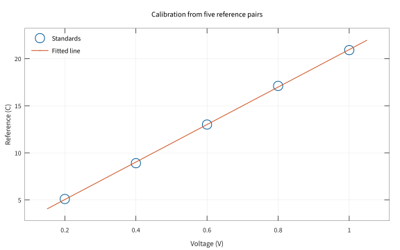
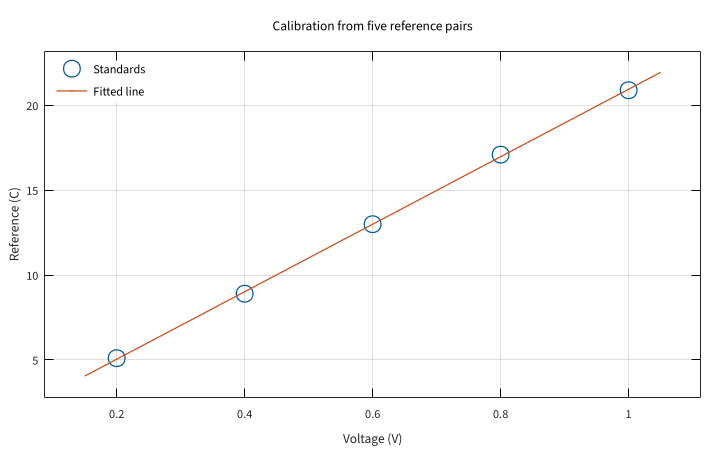
OCT-09-004

Fit a calibration line to references

A polynomial of degree one gives a gain and an offset from the paired standards. Use the fitted curve beside the observations to inspect the agreement.

Back to example overview

Compare with OCT-06-003 · Inspect a pairwise relationship.

Complete Octave source

source ("config/plot-setup.m");
voltage = [0.2 0.4 0.6 0.8 1.0]; reference = [5.1 8.9 13.0 17.1 20.9];
p = polyfit (voltage, reference, 1);
grid_voltage = linspace (0.15, 1.05, 100);
figure (1); plot (voltage, reference, "o", grid_voltage, polyval (p, grid_voltage), "-");
xlabel ("Voltage (V)"); ylabel ("Reference (C)");
key = legend ("Standards", "Fitted line", "location", "northwest");
set (key, "fontsize", 11, "box", "off");
title ("Calibration from five reference pairs"); grid on; axis padded;
printf ("Gain: %.6f C/V; offset: %.6f C\n", p(1), p(2));
print (gcf, "figures/OCT-09-004.pdf", "-dpdfcairo");
close all;
ParameterMeaning in this example
polyfit (..., 1)Estimate slope and intercept in descending-power order.
polyvalEvaluate the fitted calibration on a dense display grid.

Run this example

tools/octave examples/OCT-09-004.m > examples/OCT-09-004.stdout.txt
python3 tools/pdf_metadata.py figures/OCT-09-004.pdf
pdftocairo -svg figures/OCT-09-004.pdf figures/OCT-09-004.svg
pdftocairo -png -singlefile -r 120 figures/OCT-09-004.pdf figures/OCT-09-004

Try changing: Change one reference by 0.5 C and inspect the fitted coefficients.

Actual plot

Fit a calibration line to references
OCT-09-004 · GNU Octave / gnuplot
Gain: 19.900000 C/V; offset: 1.060000 C

GNU Octave · exit 0

Run this example
tools/octave examples/OCT-09-004.m > examples/OCT-09-004.stdout.txt
python3 tools/pdf_metadata.py figures/OCT-09-004.pdf
pdftocairo -svg figures/OCT-09-004.pdf figures/OCT-09-004.svg
pdftocairo -png -singlefile -r 120 figures/OCT-09-004.pdf figures/OCT-09-004

Download: Octave source · Source + local inputs ZIP · Captured output · SVG plot · Native PDF · PNG preview

Try changing: Change one reference by 0.5 C and inspect the fitted coefficients.

OCT-09-005

Inspect the calibration residuals

Residuals expose deviations that a fitted line can hide at the full measurement scale. Use a zero reference line and keep residuals in the original temperature unit.

Back to example overview

Compare with OCT-09-004 · Fit a calibration line to references.

Complete Octave source

source ("config/plot-setup.m");
voltage = [0.2 0.4 0.6 0.8 1.0]; reference = [5.1 8.9 13.0 17.1 20.9];
p = polyfit (voltage, reference, 1);
residual = reference - polyval (p, voltage);
figure (1); plot (voltage, residual, "o"); hold on;
plot ([0.2 1.0], [0 0], "k:");
xlabel ("Voltage (V)"); ylabel ("Residual (C)");
title ("Reference minus fitted calibration"); grid on; axis padded;
printf ("Residual sum of squares: %.6f\n", sum (residual .^ 2));
print (gcf, "figures/OCT-09-005.pdf", "-dpdfcairo");
close all;
ParameterMeaning in this example
reference minus fittedKeep the residual sign explicit.
sum (residual .^ 2)Quantify the remaining squared error.

Run this example

tools/octave examples/OCT-09-005.m > examples/OCT-09-005.stdout.txt
python3 tools/pdf_metadata.py figures/OCT-09-005.pdf
pdftocairo -svg figures/OCT-09-005.pdf figures/OCT-09-005.svg
pdftocairo -png -singlefile -r 120 figures/OCT-09-005.pdf figures/OCT-09-005

Try changing: Raise the middle reference by 0.3 C and inspect its residual.

Actual plot

Inspect the calibration residuals
OCT-09-005 · GNU Octave / gnuplot
Residual sum of squares: 0.036000

GNU Octave · exit 0

Run this example
tools/octave examples/OCT-09-005.m > examples/OCT-09-005.stdout.txt
python3 tools/pdf_metadata.py figures/OCT-09-005.pdf
pdftocairo -svg figures/OCT-09-005.pdf figures/OCT-09-005.svg
pdftocairo -png -singlefile -r 120 figures/OCT-09-005.pdf figures/OCT-09-005

Download: Octave source · Source + local inputs ZIP · Captured output · SVG plot · Native PDF · PNG preview

Try changing: Raise the middle reference by 0.3 C and inspect its residual.

OCT-09-006

Resample a repeatable set of means

Bootstrap resampling draws new samples from these six synthetic observations. Use a fixed seed and state that the displayed percentile interval is an illustrative finite-resampling result.

Back to example overview

Compare with OCT-09-001 · Distinguish spread from uncertainty of a mean.

Complete Octave source

source ("config/plot-setup.m");
readings = [11 12 12 13 14 15];
rng (17, "twister");
indices = randi (numel (readings), numel (readings), 200);
resampled_means = mean (readings(indices), 1);
interval = quantile (resampled_means, [0.05 0.95]);
figure (1); hist (resampled_means, 12);
xlabel ("Resampled mean (C)"); ylabel ("Resample count");
title ("Two hundred bootstrap means"); grid on;
printf ("Illustrative 90%% percentile interval: %.3f to %.3f C\n", interval);
print (gcf, "figures/OCT-09-006.pdf", "-dpdfcairo");
close all;
ParameterMeaning in this example
randiDraw indices with replacement from the observed values.
200 columnsConstruct two hundred resamples with six observations each.
[0.05 0.95]Retain the middle 90 percent of resampled means.

Run this example

tools/octave examples/OCT-09-006.m > examples/OCT-09-006.stdout.txt
python3 tools/pdf_metadata.py figures/OCT-09-006.pdf
pdftocairo -svg figures/OCT-09-006.pdf figures/OCT-09-006.svg
pdftocairo -png -singlefile -r 120 figures/OCT-09-006.pdf figures/OCT-09-006

Try changing: Increase the resample count to 1000 while retaining the seed.

Actual plot

Resample a repeatable set of means
OCT-09-006 · GNU Octave / gnuplot
Illustrative 90% percentile interval: 11.917 to 13.833 C

GNU Octave · exit 0

Run this example
tools/octave examples/OCT-09-006.m > examples/OCT-09-006.stdout.txt
python3 tools/pdf_metadata.py figures/OCT-09-006.pdf
pdftocairo -svg figures/OCT-09-006.pdf figures/OCT-09-006.svg
pdftocairo -png -singlefile -r 120 figures/OCT-09-006.pdf figures/OCT-09-006

Download: Octave source · Source + local inputs ZIP · Captured output · SVG plot · Native PDF · PNG preview

Try changing: Increase the resample count to 1000 while retaining the seed.

10 · Numerical methods

Choose a numerical method for the mathematical question and state its domain. Compare against an analytic result when one is available, and keep tolerances and brackets explicit.

OCT-10-001

Interpolate between observations

Interpolation supplies values between the four observed times without fitting a global calibration law. Use a named method and keep the measured points visible.

Back to example overview

Compare with OCT-06-001 · Compare two sensor runs.

Complete Octave source

source ("config/plot-setup.m");
hours = [0 2 4 6]; readings = [12 15 13 17];
fine_hours = linspace (0, 6, 121);
interpolated = interp1 (hours, readings, fine_hours, "linear");
figure (1); plot (hours, readings, "o", fine_hours, interpolated, "-");
xlabel ("Time (hours)"); ylabel ("Reading (C)");
key = legend ("Observed", "Interpolated", "location", "northwest");
set (key, "fontsize", 11, "box", "off");
title ("Interpolate inside the observed interval"); grid on; axis padded;
printf ("Reading at hour 1: %.3f C\n", interp1 (hours, readings, 1, "linear"));
print (gcf, "figures/OCT-10-001.pdf", "-dpdfcairo");
close all;
ParameterMeaning in this example
interp1 (..., "linear")Interpolate within the observed time interval.
Observed markersDistinguish measurements from interpolated values.

Run this example

tools/octave examples/OCT-10-001.m > examples/OCT-10-001.stdout.txt
python3 tools/pdf_metadata.py figures/OCT-10-001.pdf
pdftocairo -svg figures/OCT-10-001.pdf figures/OCT-10-001.svg
pdftocairo -png -singlefile -r 120 figures/OCT-10-001.pdf figures/OCT-10-001

Try changing: Replace linear with pchip and compare the curve.

Actual plot

Interpolate between observations
OCT-10-001 · GNU Octave / gnuplot
Reading at hour 1: 13.500 C

GNU Octave · exit 0

Run this example
tools/octave examples/OCT-10-001.m > examples/OCT-10-001.stdout.txt
python3 tools/pdf_metadata.py figures/OCT-10-001.pdf
pdftocairo -svg figures/OCT-10-001.pdf figures/OCT-10-001.svg
pdftocairo -png -singlefile -r 120 figures/OCT-10-001.pdf figures/OCT-10-001

Download: Octave source · Source + local inputs ZIP · Captured output · SVG plot · Native PDF · PNG preview

Try changing: Replace linear with pchip and compare the curve.

OCT-10-002

Integrate a sampled rate

The trapezoidal rule integrates values recorded at known times. Use the actual time vector so irregular observation spacing would be respected.

Back to example overview

Compare with OCT-10-001 · Interpolate between observations.

Complete Octave source

hours = [0 1 2 3]; rate = [0 2 2 0];
integrated = trapz (hours, rate);
printf ("Integrated signal: %.3f unit-hours\n", integrated);
ParameterMeaning in this example
trapz (hours, rate)Add the areas of consecutive trapezoids.
unit-hoursMultiply the rate unit by the time unit.

Run this example

tools/octave examples/OCT-10-002.m > examples/OCT-10-002.stdout.txt

Try changing: Change the final time to 4 while keeping its rate zero.

Actual numerical result

Integrated signal: 4.000 unit-hours

GNU Octave · exit 0

Run this example
tools/octave examples/OCT-10-002.m > examples/OCT-10-002.stdout.txt

Download: Octave source · Source + local inputs ZIP · Captured output

Try changing: Change the final time to 4 while keeping its rate zero.

OCT-10-003

Integrate a continuous response

Adaptive quadrature evaluates a function over the stated interval. Use the analytic exponential integral to check the numerical result.

Back to example overview

Compare with OCT-10-002 · Integrate a sampled rate.

Complete Octave source

response = @(t) exp (-t);
[area, estimated_error] = quadgk (response, 0, 4);
exact = 1 - exp (-4);
printf ("Integral: %.12f; analytic: %.12f\n", area, exact);
printf ("Estimated error: %.3g\n", estimated_error);
ParameterMeaning in this example
quadgkAdaptively integrate the supplied function handle.
1-exp(-4)State the independent analytic reference.

Run this example

tools/octave examples/OCT-10-003.m > examples/OCT-10-003.stdout.txt

Try changing: Change the upper limit to 6 in both calculations.

Actual numerical result

Integral: 0.981684361111; analytic: 0.981684361111
Estimated error: 6.92e-14

GNU Octave · exit 0

Run this example
tools/octave examples/OCT-10-003.m > examples/OCT-10-003.stdout.txt

Download: Octave source · Source + local inputs ZIP · Captured output

Try changing: Change the upper limit to 6 in both calculations.

OCT-10-004

Locate a threshold crossing

A bracketed root search finds when the decaying response reaches 0.2. Use a bracket that contains the crossing instead of an unexplained initial guess.

Back to example overview

Compare with OCT-10-003 · Integrate a continuous response.

Complete Octave source

threshold_difference = @(t) exp (-t) - 0.2;
crossing = fzero (threshold_difference, [0 4]);
printf ("Crossing: %.9f hours; residual: %.9f\n", ...
        crossing, threshold_difference (crossing));
ParameterMeaning in this example
[0 4]Bracket the crossing within the stated time domain.
fzeroFind a zero of response minus threshold.

Run this example

tools/octave examples/OCT-10-004.m > examples/OCT-10-004.stdout.txt

Try changing: Change the threshold from 0.2 to 0.1 and predict the direction of the shift.

Actual numerical result

Crossing: 1.609437912 hours; residual: -0.000000000

GNU Octave · exit 0

Run this example
tools/octave examples/OCT-10-004.m > examples/OCT-10-004.stdout.txt

Download: Octave source · Source + local inputs ZIP · Captured output

Try changing: Change the threshold from 0.2 to 0.1 and predict the direction of the shift.

OCT-10-005

Minimize a bounded mismatch score

A bounded minimizer searches this synthetic one-parameter score. Use the known quadratic minimum to make the result easy to assess.

Back to example overview

Compare with OCT-10-004 · Locate a threshold crossing.

Complete Octave source

source ("config/plot-setup.m");
score = @(setting) (setting - 2.4).^2 + 0.3;
best = fminbnd (score, 0, 5);
settings = linspace (0, 5, 101);
figure (1); plot (settings, score (settings)); hold on;
plot (best, score (best), "o");
xlabel ("Setting"); ylabel ("Mismatch score");
title ("Search a bounded one-parameter score"); grid on; axis padded;
printf ("Best setting: %.6f; score: %.6f\n", best, score (best));
print (gcf, "figures/OCT-10-005.pdf", "-dpdfcairo");
close all;
ParameterMeaning in this example
fminbnd (..., 0, 5)Search only inside the permitted interval.
2.4 / 0.3Identify the known position and value of this quadratic minimum.

Run this example

tools/octave examples/OCT-10-005.m > examples/OCT-10-005.stdout.txt
python3 tools/pdf_metadata.py figures/OCT-10-005.pdf
pdftocairo -svg figures/OCT-10-005.pdf figures/OCT-10-005.svg
pdftocairo -png -singlefile -r 120 figures/OCT-10-005.pdf figures/OCT-10-005

Try changing: Move the known minimum to 3.2 and compare the result.

Actual plot

Minimize a bounded mismatch score
OCT-10-005 · GNU Octave / gnuplot
Best setting: 2.400000; score: 0.300000

GNU Octave · exit 0

Run this example
tools/octave examples/OCT-10-005.m > examples/OCT-10-005.stdout.txt
python3 tools/pdf_metadata.py figures/OCT-10-005.pdf
pdftocairo -svg figures/OCT-10-005.pdf figures/OCT-10-005.svg
pdftocairo -png -singlefile -r 120 figures/OCT-10-005.pdf figures/OCT-10-005

Download: Octave source · Source + local inputs ZIP · Captured output · SVG plot · Native PDF · PNG preview

Try changing: Move the known minimum to 3.2 and compare the result.

OCT-10-006

Check a differential-equation solution

An adaptive solver evolves a normalized response from its initial value. Use requested output times and an analytic solution to assess the complete trajectory.

Back to example overview

Compare with OCT-07-001 · Inspect exponential decay on a log scale.

Complete Octave source

source ("config/plot-setup.m");
times = (0:0.5:5).';
options = odeset ("RelTol", 1e-8, "AbsTol", 1e-10);
[t, response] = ode45 (@(t, value) -0.5 .* value, times, 1, options);
exact = exp (-0.5 .* t);
figure (1); plot (t, response, "o", t, exact, "-");
xlabel ("Time (hours)"); ylabel ("Normalized response");
key = legend ("ode45", "Analytic", "location", "northeast");
set (key, "fontsize", 11, "box", "off");
title ("Check an adaptive decay solution"); grid on; axis padded;
printf ("Final response: %.9f; maximum error: %.3g\n", response(end), max (abs (response - exact)));
print (gcf, "figures/OCT-10-006.pdf", "-dpdfcairo");
close all;
ParameterMeaning in this example
ode45Solve the stated initial-value problem.
odesetState relative and absolute error tolerances.
exp (-0.5 .* t)Check against the analytic trajectory at every requested time.

Run this example

tools/octave examples/OCT-10-006.m > examples/OCT-10-006.stdout.txt
python3 tools/pdf_metadata.py figures/OCT-10-006.pdf
pdftocairo -svg figures/OCT-10-006.pdf figures/OCT-10-006.svg
pdftocairo -png -singlefile -r 120 figures/OCT-10-006.pdf figures/OCT-10-006

Try changing: Change the decay coefficient to 0.8 in the solver and analytic reference.

Actual plot

Check a differential-equation solution
OCT-10-006 · GNU Octave / gnuplot
Final response: 0.082084999; maximum error: 8.26e-10

GNU Octave · exit 0

Run this example
tools/octave examples/OCT-10-006.m > examples/OCT-10-006.stdout.txt
python3 tools/pdf_metadata.py figures/OCT-10-006.pdf
pdftocairo -svg figures/OCT-10-006.pdf figures/OCT-10-006.svg
pdftocairo -png -singlefile -r 120 figures/OCT-10-006.pdf figures/OCT-10-006

Download: Octave source · Source + local inputs ZIP · Captured output · SVG plot · Native PDF · PNG preview

Try changing: Change the decay coefficient to 0.8 in the solver and analytic reference.

11 · Files and sampled signals

Read a complete local fixture and preserve its schema when exporting results. For sampled signals, state the sample rate, normalization and treatment of boundaries.

OCT-11-001

Read the local monitoring batch

A numeric CSV reader imports the twelve-row synthetic fixture after its header. Use an explicit skipped-header count and inspect the dimensions before selecting fields.

Back to example overview

Compare with OCT-01-004 · Arrange readings in a matrix.

Complete Octave source

batch = dlmread ("data/monitoring.csv", ",", 1, 0);
printf ("Rows: %d; columns: %d\n", rows (batch), columns (batch));
printf ("First site: %d; final voltage: %.2f V\n", batch(1,1), batch(end,3));
ParameterMeaning in this example
dlmread (..., ",", 1, 0)Skip one header row and start at the first numeric column.
[site hour voltage quality]Keep the four-column local schema explicit.

Run this example

tools/octave examples/OCT-11-001.m > examples/OCT-11-001.stdout.txt

Try changing: Inspect the voltage column and identify its missing value.

Actual numerical result

Rows: 12; columns: 4
First site: 1; final voltage: 0.95 V

GNU Octave · exit 0

Run this example
tools/octave examples/OCT-11-001.m > examples/OCT-11-001.stdout.txt

Download: Octave source · Source + local inputs ZIP · Captured output

Try changing: Inspect the voltage column and identify its missing value.

OCT-11-002

Round-trip a native numerical array

Octave’s binary format preserves an array without a text creation-date header. Use a named loaded structure so the restored value cannot silently replace another workspace variable.

Back to example overview

Compare with OCT-11-001 · Read the local monitoring batch.

Complete Octave source

readings = [11 13 15];
save ("-binary", "generated/OCT-11-002.bin", "readings");
restored = load ("generated/OCT-11-002.bin");
printf ("Restored values: %d; total: %.3f C\n", ...
        numel (restored.readings), sum (restored.readings));
ParameterMeaning in this example
"-binary"Use Octave’s native binary array format.
restored.readingsRead the named field from the loaded structure.

Run this example

tools/octave examples/OCT-11-002.m > examples/OCT-11-002.stdout.txt

Try changing: Save and restore a two-row matrix instead.

Actual numerical result

Restored values: 3; total: 39.000 C

GNU Octave · exit 0

Run this example
tools/octave examples/OCT-11-002.m > examples/OCT-11-002.stdout.txt

Download: Octave source · Source + local inputs ZIP · Captured output · OCT-11-002.bin

Try changing: Save and restore a two-row matrix instead.

OCT-11-003

Export a structured record as JSON

JSON carries the site identifier and its reading array into another tool. Use encode and decode together to check that the exported record retains the expected content.

Back to example overview

Compare with OCT-11-002 · Round-trip a native numerical array.

Complete Octave source

record = struct ("site", 2, "readings_C", [14 15 16]);
text = jsonencode (record);
fid = fopen ("generated/OCT-11-003.json", "w");
fprintf (fid, "%s\n", text); fclose (fid);
restored = jsondecode (text);
printf ("%s\nRestored total: %.3f C\n", text, sum (restored.readings_C));
ParameterMeaning in this example
jsonencode / jsondecodeSerialize and recover a complete structured record.
fopen / fprintf / fcloseWrite that exact JSON to the named local output.

Run this example

tools/octave examples/OCT-11-003.m > examples/OCT-11-003.stdout.txt

Try changing: Add a unit field and verify it after decoding.

Actual numerical result

{"site":2,"readings_C":[14,15,16]}
Restored total: 45.000 C

GNU Octave · exit 0

Run this example
tools/octave examples/OCT-11-003.m > examples/OCT-11-003.stdout.txt

Download: Octave source · Source + local inputs ZIP · Captured output · OCT-11-003.json

Try changing: Add a unit field and verify it after decoding.

OCT-11-004

Locate a known frequency with an FFT

A synthetic five-hertz sinusoid supplies an exact frequency reference. Use the stated sample rate and single-sided amplitude normalization to keep the spectrum interpretable.

Back to example overview

Compare with OCT-11-003 · Export a structured record as JSON.

Complete Octave source

source ("config/plot-setup.m");
N = 128; sample_rate = 32;
time = (0:N-1) ./ sample_rate;
signal = sin (2 .* pi .* 5 .* time);
transformed = fft (signal);
amplitude = 2 .* abs (transformed(1:N/2+1)) ./ N;
amplitude([1 end]) = amplitude([1 end]) ./ 2;
frequency = (0:N/2) .* sample_rate ./ N;
figure (1); stem (frequency, amplitude);
xlabel ("Frequency (Hz)"); ylabel ("Single-sided amplitude");
title ("Find the synthetic five-hertz component"); grid on; axis padded;
[peak, index] = max (amplitude);
printf ("Peak: %.3f Hz; amplitude: %.6f\n", frequency(index), peak);
print (gcf, "figures/OCT-11-004.pdf", "-dpdfcairo");
close all;
ParameterMeaning in this example
fftTransform the complete 128-sample signal.
sample_rate = 32Set sample spacing and the frequency axis.
Single-sided normalizationDouble interior amplitudes but not DC or the Nyquist endpoint.

Run this example

tools/octave examples/OCT-11-004.m > examples/OCT-11-004.stdout.txt
python3 tools/pdf_metadata.py figures/OCT-11-004.pdf
pdftocairo -svg figures/OCT-11-004.pdf figures/OCT-11-004.svg
pdftocairo -png -singlefile -r 120 figures/OCT-11-004.pdf figures/OCT-11-004

Try changing: Change the known component to 7 Hz.

Actual plot

Locate a known frequency with an FFT
OCT-11-004 · GNU Octave / gnuplot
Peak: 5.000 Hz; amplitude: 1.000000

GNU Octave · exit 0

Run this example
tools/octave examples/OCT-11-004.m > examples/OCT-11-004.stdout.txt
python3 tools/pdf_metadata.py figures/OCT-11-004.pdf
pdftocairo -svg figures/OCT-11-004.pdf figures/OCT-11-004.svg
pdftocairo -png -singlefile -r 120 figures/OCT-11-004.pdf figures/OCT-11-004

Download: Octave source · Source + local inputs ZIP · Captured output · SVG plot · Native PDF · PNG preview

Try changing: Change the known component to 7 Hz.

OCT-11-005

Smooth only fully observed windows

A three-point convolution averages neighboring observations. Use valid mode to omit edge windows that would otherwise require assumed samples beyond the run.

Back to example overview

Compare with OCT-11-004 · Locate a known frequency with an FFT.

Complete Octave source

source ("config/plot-setup.m");
readings = [12 14 13 16 15 17 14];
smoothed = conv (readings, ones (1,3) ./ 3, "valid");
figure (1); plot (1:7, readings, "-o", 2:6, smoothed, "-s");
xlabel ("Observation index"); ylabel ("Reading (C)");
key = legend ("Observed", "Three-point mean", "location", "northwest");
set (key, "fontsize", 11, "box", "off");
title ("Average complete three-point windows"); grid on; axis padded;
printf ("Smoothed:"); printf (" %.3f", smoothed); printf ("\n");
print (gcf, "figures/OCT-11-005.pdf", "-dpdfcairo");
close all;
ParameterMeaning in this example
conv (..., "valid")Keep only windows fully covered by observations.
2:6Place each average at its original center observation.

Run this example

tools/octave examples/OCT-11-005.m > examples/OCT-11-005.stdout.txt
python3 tools/pdf_metadata.py figures/OCT-11-005.pdf
pdftocairo -svg figures/OCT-11-005.pdf figures/OCT-11-005.svg
pdftocairo -png -singlefile -r 120 figures/OCT-11-005.pdf figures/OCT-11-005

Try changing: Use a five-point kernel and adjust its center indices.

Actual plot

Smooth only fully observed windows
OCT-11-005 · GNU Octave / gnuplot
Smoothed: 13.000 14.333 14.667 16.000 15.333

GNU Octave · exit 0

Run this example
tools/octave examples/OCT-11-005.m > examples/OCT-11-005.stdout.txt
python3 tools/pdf_metadata.py figures/OCT-11-005.pdf
pdftocairo -svg figures/OCT-11-005.pdf figures/OCT-11-005.svg
pdftocairo -png -singlefile -r 120 figures/OCT-11-005.pdf figures/OCT-11-005

Download: Octave source · Source + local inputs ZIP · Captured output · SVG plot · Native PDF · PNG preview

Try changing: Use a five-point kernel and adjust its center indices.

OCT-11-006

Track cumulative arrivals

A cumulative sum turns completed hourly counts into an intake total. Use counts rather than sampled rates so the accumulation has an unambiguous interpretation.

Back to example overview

Compare with OCT-11-005 · Smooth only fully observed windows.

Complete Octave source

source ("config/plot-setup.m");
arrivals = [2 1 3 2];
total = cumsum (arrivals);
figure (1); stairs (0:4, [0 total]);
xlabel ("Completed hour"); ylabel ("Cumulative samples");
title ("Accumulate four hourly intake counts"); grid on; axis padded;
printf ("Cumulative:"); printf (" %d", total); printf ("\n");
print (gcf, "figures/OCT-11-006.pdf", "-dpdfcairo");
close all;
ParameterMeaning in this example
cumsumAdd each completed hourly count to the previous total.
stairsShow changes at discrete hour boundaries.

Run this example

tools/octave examples/OCT-11-006.m > examples/OCT-11-006.stdout.txt
python3 tools/pdf_metadata.py figures/OCT-11-006.pdf
pdftocairo -svg figures/OCT-11-006.pdf figures/OCT-11-006.svg
pdftocairo -png -singlefile -r 120 figures/OCT-11-006.pdf figures/OCT-11-006

Try changing: Increase only the third hourly count from 3 to 5.

Actual plot

Track cumulative arrivals
OCT-11-006 · GNU Octave / gnuplot
Cumulative: 2 3 6 8

GNU Octave · exit 0

Run this example
tools/octave examples/OCT-11-006.m > examples/OCT-11-006.stdout.txt
python3 tools/pdf_metadata.py figures/OCT-11-006.pdf
pdftocairo -svg figures/OCT-11-006.pdf figures/OCT-11-006.svg
pdftocairo -png -singlefile -r 120 figures/OCT-11-006.pdf figures/OCT-11-006

Download: Octave source · Source + local inputs ZIP · Captured output · SVG plot · Native PDF · PNG preview

Try changing: Increase only the third hourly count from 3 to 5.

12 · One field investigation in six steps

Follow the same twelve-row synthetic batch from input inspection to a downloadable summary. Each program starts again from the local CSV so every step remains independently reproducible.

OCT-12-001

Inspect the batch before analysis

The first pass checks the local schema and identifies flagged or nonfinite observations. Use those counts to decide which cleaning rule the next calculation must state.

Back to example overview

Compare with OCT-11-001 · Read the local monitoring batch.

Complete Octave source

batch = dlmread ("data/monitoring.csv", ",", 1, 0);
printf ("Rows: %d; fields: %d; sites: %d\n", ...
        rows (batch), columns (batch), numel (unique (batch(:,1))));
printf ("Flagged rows: %d; nonfinite voltages: %d\n", ...
        sum (batch(:,4) == 0), sum (! isfinite (batch(:,3))));
ParameterMeaning in this example
unique (site)Count the distinct collection identifiers.
Quality / finiteness countsInspect both rejection reasons before filtering.

Run this example

tools/octave examples/OCT-12-001.m > examples/OCT-12-001.stdout.txt

Try changing: Change one quality flag in a copy of the CSV and rerun this inspection.

Actual numerical result

Rows: 12; fields: 4; sites: 3
Flagged rows: 2; nonfinite voltages: 1

GNU Octave · exit 0

Run this example
tools/octave examples/OCT-12-001.m > examples/OCT-12-001.stdout.txt

Download: Octave source · Source + local inputs ZIP · Captured output

Try changing: Change one quality flag in a copy of the CSV and rerun this inspection.

OCT-12-002

Apply a visible acceptance rule

A reading is accepted only when its quality flag is one and its voltage is finite. Use the same mask for every retained column to preserve the observation rows.

Back to example overview

Compare with OCT-12-001 · Inspect the batch before analysis.

Complete Octave source

batch = dlmread ("data/monitoring.csv", ",", 1, 0);
accepted = batch(:,4) == 1 & isfinite (batch(:,3));
clean = batch(accepted, :);
printf ("Accepted: %d; rejected: %d\n", rows (clean), rows (batch) - rows (clean));
printf ("Accepted mean voltage: %.4f V\n", mean (clean(:,3)));
ParameterMeaning in this example
&Require the quality and finiteness tests for every row.
batch(accepted, :)Apply one complete row mask to all fields.

Run this example

tools/octave examples/OCT-12-002.m > examples/OCT-12-002.stdout.txt

Try changing: Add an upper accepted voltage limit of 0.85 V.

Actual numerical result

Accepted: 10; rejected: 2
Accepted mean voltage: 0.7250 V

GNU Octave · exit 0

Run this example
tools/octave examples/OCT-12-002.m > examples/OCT-12-002.stdout.txt

Download: Octave source · Source + local inputs ZIP · Captured output

Try changing: Add an upper accepted voltage limit of 0.85 V.

OCT-12-003

Calibrate the accepted observations

Three exact synthetic standards define the voltage-to-temperature conversion. Use that fit only after rejecting invalid observations, and keep the standards separate from the monitoring batch.

Back to example overview

Compare with OCT-09-004 · Fit a calibration line to references.

Complete Octave source

source ("config/plot-setup.m");
batch = dlmread ("data/monitoring.csv", ",", 1, 0);
clean = batch(batch(:,4) == 1 & isfinite (batch(:,3)), :);
p = polyfit ([0 0.5 1], [1 11 21], 1);
temperature = polyval (p, clean(:,3));
figure (1); scatter (clean(:,3), temperature, 40, "filled");
xlabel ("Accepted voltage (V)"); ylabel ("Calibrated reading (C)");
title ("Convert the accepted field observations"); grid on; axis padded;
printf ("Gain: %.3f; offset: %.3f; mean: %.3f C\n", p(1), p(2), mean (temperature));
print (gcf, "figures/OCT-12-003.pdf", "-dpdfcairo");
close all;
ParameterMeaning in this example
Separate standardsUse the three stated reference pairs to fit the calibration.
polyval (p, clean(:,3))Convert only accepted batch voltages.

Run this example

tools/octave examples/OCT-12-003.m > examples/OCT-12-003.stdout.txt
python3 tools/pdf_metadata.py figures/OCT-12-003.pdf
pdftocairo -svg figures/OCT-12-003.pdf figures/OCT-12-003.svg
pdftocairo -png -singlefile -r 120 figures/OCT-12-003.pdf figures/OCT-12-003

Try changing: Change the reference offset from 1 C to 2 C in all three standards.

Actual plot

Calibrate the accepted observations
OCT-12-003 · GNU Octave / gnuplot
Gain: 20.000; offset: 1.000; mean: 15.500 C

GNU Octave · exit 0

Run this example
tools/octave examples/OCT-12-003.m > examples/OCT-12-003.stdout.txt
python3 tools/pdf_metadata.py figures/OCT-12-003.pdf
pdftocairo -svg figures/OCT-12-003.pdf figures/OCT-12-003.svg
pdftocairo -png -singlefile -r 120 figures/OCT-12-003.pdf figures/OCT-12-003

Download: Octave source · Source + local inputs ZIP · Captured output · SVG plot · Native PDF · PNG preview

Try changing: Change the reference offset from 1 C to 2 C in all three standards.

OCT-12-004

Summarize accepted readings by site

Grouping applies the same mean calculation independently to each site. Use site identifiers as the accumulation indices and report how many observations support each mean.

Back to example overview

Compare with OCT-06-004 · Compare site summaries with bars.

Complete Octave source

source ("config/plot-setup.m");
batch = dlmread ("data/monitoring.csv", ",", 1, 0);
clean = batch(batch(:,4) == 1 & isfinite (batch(:,3)), :);
temperature = 20 .* clean(:,3) + 1;
site_mean = accumarray (clean(:,1), temperature, [], @mean);
site_count = accumarray (clean(:,1), 1);
figure (1); bar (1:3, site_mean); set (gca, "xtick", 1:3);
xlabel ("Site identifier"); ylabel ("Mean accepted reading (C)");
title ("Site summaries after quality checks"); grid on;
for site = 1:3
  printf ("Site %d: n=%d; mean=%.3f C\n", site, site_count(site), site_mean(site));
endfor
print (gcf, "figures/OCT-12-004.pdf", "-dpdfcairo");
close all;
ParameterMeaning in this example
accumarray (..., @mean)Calculate one mean per site index.
accumarray (..., 1)Count accepted observations in the same groups.

Run this example

tools/octave examples/OCT-12-004.m > examples/OCT-12-004.stdout.txt
python3 tools/pdf_metadata.py figures/OCT-12-004.pdf
pdftocairo -svg figures/OCT-12-004.pdf figures/OCT-12-004.svg
pdftocairo -png -singlefile -r 120 figures/OCT-12-004.pdf figures/OCT-12-004

Try changing: Calculate the maximum per site with @max while retaining the counts.

Actual plot

Summarize accepted readings by site
OCT-12-004 · GNU Octave / gnuplot
Site 1: n=3; mean=12.000 C
Site 2: n=3; mean=15.000 C
Site 3: n=4; mean=18.500 C

GNU Octave · exit 0

Run this example
tools/octave examples/OCT-12-004.m > examples/OCT-12-004.stdout.txt
python3 tools/pdf_metadata.py figures/OCT-12-004.pdf
pdftocairo -svg figures/OCT-12-004.pdf figures/OCT-12-004.svg
pdftocairo -png -singlefile -r 120 figures/OCT-12-004.pdf figures/OCT-12-004

Download: Octave source · Source + local inputs ZIP · Captured output · SVG plot · Native PDF · PNG preview

Try changing: Calculate the maximum per site with @max while retaining the counts.

OCT-12-005

Fit a trend within one site

A time trend must refer to a defined site rather than a mixture of site levels. Use the accepted observations from site one and keep its fitted slope in temperature per hour.

Back to example overview

Compare with OCT-08-002 · Fit an overdetermined linear model.

Complete Octave source

source ("config/plot-setup.m");
batch = dlmread ("data/monitoring.csv", ",", 1, 0);
selected = batch(:,1) == 1 & batch(:,4) == 1 & isfinite (batch(:,3));
hours = batch(selected, 2); temperature = 20 .* batch(selected, 3) + 1;
p = polyfit (hours, temperature, 1);
fine_hours = linspace (min (hours), max (hours), 50);
figure (1); plot (hours, temperature, "o", fine_hours, polyval (p, fine_hours), "-");
xlabel ("Time (hours)"); ylabel ("Site one reading (C)");
title ("Fit within one collection site"); grid on; axis padded;
printf ("Site one slope: %.6f C/hour; intercept: %.6f C\n", p(1), p(2));
print (gcf, "figures/OCT-12-005.pdf", "-dpdfcairo");
close all;
ParameterMeaning in this example
Site-one maskHold the collection site fixed before fitting time.
Slope unitReport C per hour rather than a unitless coefficient.

Run this example

tools/octave examples/OCT-12-005.m > examples/OCT-12-005.stdout.txt
python3 tools/pdf_metadata.py figures/OCT-12-005.pdf
pdftocairo -svg figures/OCT-12-005.pdf figures/OCT-12-005.svg
pdftocairo -png -singlefile -r 120 figures/OCT-12-005.pdf figures/OCT-12-005

Try changing: Select site two and compare its slope and intercept.

Actual plot

Fit a trend within one site
OCT-12-005 · GNU Octave / gnuplot
Site one slope: 1.000000 C/hour; intercept: 11.000000 C

GNU Octave · exit 0

Run this example
tools/octave examples/OCT-12-005.m > examples/OCT-12-005.stdout.txt
python3 tools/pdf_metadata.py figures/OCT-12-005.pdf
pdftocairo -svg figures/OCT-12-005.pdf figures/OCT-12-005.svg
pdftocairo -png -singlefile -r 120 figures/OCT-12-005.pdf figures/OCT-12-005

Download: Octave source · Source + local inputs ZIP · Captured output · SVG plot · Native PDF · PNG preview

Try changing: Select site two and compare its slope and intercept.

OCT-12-006

Export the complete batch summary

A structured summary records the acceptance count and site means alongside the plot. Use the same explicit quality rule for both outputs so the downloaded JSON and figure describe the same observations.

Back to example overview

Compare with OCT-11-003 · Export a structured record as JSON.

Complete Octave source

source ("config/plot-setup.m");
batch = dlmread ("data/monitoring.csv", ",", 1, 0);
clean = batch(batch(:,4) == 1 & isfinite (batch(:,3)), :);
temperature = 20 .* clean(:,3) + 1;
site_mean = accumarray (clean(:,1), temperature, [], @mean);
summary = struct ("rows", rows(batch), "accepted", rows(clean), ...
                  "sites", [1 2 3], "mean_C", site_mean.');
fid = fopen ("generated/OCT-12-006-summary.json", "w");
fprintf (fid, "%s\n", jsonencode (summary)); fclose (fid);
figure (1); bar (1:3, site_mean); set (gca, "xtick", 1:3);
xlabel ("Site identifier"); ylabel ("Mean accepted reading (C)");
title ("A reproducible field-batch summary"); grid on;
printf ("Summary rows: %d; accepted: %d; overall mean: %.3f C\n", ...
        rows (batch), rows (clean), mean (temperature));
print (gcf, "figures/OCT-12-006.pdf", "-dpdfcairo");
close all;
ParameterMeaning in this example
summaryRetain input count, accepted count and site means in one record.
jsonencode / fprintfExport the same computed values as local JSON.

Run this example

tools/octave examples/OCT-12-006.m > examples/OCT-12-006.stdout.txt
python3 tools/pdf_metadata.py figures/OCT-12-006.pdf
pdftocairo -svg figures/OCT-12-006.pdf figures/OCT-12-006.svg
pdftocairo -png -singlefile -r 120 figures/OCT-12-006.pdf figures/OCT-12-006

Try changing: Add the rejected count and a unit field to the JSON summary.

Actual plot

Export the complete batch summary
OCT-12-006 · GNU Octave / gnuplot
Summary rows: 12; accepted: 10; overall mean: 15.500 C

GNU Octave · exit 0

Run this example
tools/octave examples/OCT-12-006.m > examples/OCT-12-006.stdout.txt
python3 tools/pdf_metadata.py figures/OCT-12-006.pdf
pdftocairo -svg figures/OCT-12-006.pdf figures/OCT-12-006.svg
pdftocairo -png -singlefile -r 120 figures/OCT-12-006.pdf figures/OCT-12-006

Download: Octave source · Source + local inputs ZIP · Captured output · SVG plot · Native PDF · PNG preview · OCT-12-006-summary.json

Try changing: Add the rejected count and a unit field to the JSON summary.

13 · Axes, scales and sampling

Control what the viewer can infer from a curve: sampling, gaps, ticks, orientation, logarithmic scales and fixed calendar coordinates. Compare every technique with its gnuplot counterpart.

OCT-13-001

Expose the effect of coarse sampling

A fast oscillation can look like a slow one when too few coordinates are evaluated. Compare two explicit grids over the same time interval before interpreting a sampled curve.

Back to example overview

Compare with OCT-01-006 · Plot the first measurements.

Compare with gnuplot · Increase samples without changing the function.

Complete Octave source

source ("config/plot-setup.m");
coarse = linspace (0, 2, 9); fine = linspace (0, 2, 401);
response = @(t) sin (2*pi*3*t);
figure (1); plot (fine, response(fine), "-", coarse, response(coarse), "o--");
xlabel ("Time (hours)"); ylabel ("Synthetic response");
title ("Sampling can hide an oscillation"); grid on; axis padded;
key = legend ("401 coordinates", "9 coordinates", "location", "southoutside");
set (key, "fontsize", 11, "box", "off");
printf ("Coarse interval: %.3f hours; signal period: %.3f hours\n", ...
        coarse(2)-coarse(1), 1/3);
print (gcf, "figures/OCT-13-001.pdf", "-dpdfcairo");
close all;
ParameterMeaning in this example
linspace (..., 9 / 401)Compare sparse and dense coordinates for the same function.
2*pi*3*tUse three cycles per hour; the phase is in radians.

Run this example

tools/octave examples/OCT-13-001.m > examples/OCT-13-001.stdout.txt
python3 tools/pdf_metadata.py figures/OCT-13-001.pdf
pdftocairo -svg figures/OCT-13-001.pdf figures/OCT-13-001.svg
pdftocairo -png -singlefile -r 120 figures/OCT-13-001.pdf figures/OCT-13-001

Try changing: Change the coarse grid to 25 coordinates.

Actual plot

Expose the effect of coarse sampling
OCT-13-001 · GNU Octave / gnuplot
Coarse interval: 0.250 hours; signal period: 0.333 hours

GNU Octave · exit 0

Run this example
tools/octave examples/OCT-13-001.m > examples/OCT-13-001.stdout.txt
python3 tools/pdf_metadata.py figures/OCT-13-001.pdf
pdftocairo -svg figures/OCT-13-001.pdf figures/OCT-13-001.svg
pdftocairo -png -singlefile -r 120 figures/OCT-13-001.pdf figures/OCT-13-001

Download: Octave source · Source + local inputs ZIP · Captured output · SVG plot · Native PDF · PNG preview

Try changing: Change the coarse grid to 25 coordinates.

OCT-13-002

Break a curve at an excluded interval

A missing interval should remain a gap rather than an invented connecting segment. Assign NaN to the excluded samples while keeping their original coordinates.

Back to example overview

Compare with OCT-02-005 · Replace flagged values in place.

Compare with gnuplot · Break a line at an excluded interval.

Complete Octave source

source ("config/plot-setup.m");
hours = 0:0.05:6; readings = 13 + sin (hours);
excluded = hours >= 2 & hours <= 3;
readings(excluded) = NaN;
figure (1); plot (hours, readings, "-");
xlabel ("Time (hours)"); ylabel ("Reading (C)");
title ("Do not join across an unobserved interval"); grid on;
xlim ([0 6]); ylim ([11.5 14.5]);
printf ("Excluded coordinates: %d\n", sum (excluded));
print (gcf, "figures/OCT-13-002.pdf", "-dpdfcairo");
close all;
ParameterMeaning in this example
NaNBreak the native line at excluded observations.
hours >= 2 & hours <= 3Define an inclusive one-hour exclusion interval.

Run this example

tools/octave examples/OCT-13-002.m > examples/OCT-13-002.stdout.txt
python3 tools/pdf_metadata.py figures/OCT-13-002.pdf
pdftocairo -svg figures/OCT-13-002.pdf figures/OCT-13-002.svg
pdftocairo -png -singlefile -r 120 figures/OCT-13-002.pdf figures/OCT-13-002

Try changing: Move the excluded interval to hours 4 through 5.

Actual plot

Break a curve at an excluded interval
OCT-13-002 · GNU Octave / gnuplot
Excluded coordinates: 21

GNU Octave · exit 0

Run this example
tools/octave examples/OCT-13-002.m > examples/OCT-13-002.stdout.txt
python3 tools/pdf_metadata.py figures/OCT-13-002.pdf
pdftocairo -svg figures/OCT-13-002.pdf figures/OCT-13-002.svg
pdftocairo -png -singlefile -r 120 figures/OCT-13-002.pdf figures/OCT-13-002

Download: Octave source · Source + local inputs ZIP · Captured output · SVG plot · Native PDF · PNG preview

Try changing: Move the excluded interval to hours 4 through 5.

OCT-13-003

Place named ticks at irregular coordinates

Tick positions and tick labels are independent properties. Name collection visits at their actual unequal time intervals instead of spacing them as categories.

Back to example overview

Compare with OCT-13-002 · Break a curve at an excluded interval.

Compare with gnuplot · Choose irregular tick positions.

Complete Octave source

source ("config/plot-setup.m");
hours = [0 1 3 6]; readings = [12 14 13 17];
figure (1); plot (hours, readings, "o-");
set (gca, "xtick", hours, "xticklabel", {"Start", "Visit A", "Visit B", "End"});
xlabel ("Unequally spaced visits"); ylabel ("Reading (C)");
title ("Named ticks keep their measured positions"); grid on; axis padded;
print (gcf, "figures/OCT-13-003.pdf", "-dpdfcairo");
close all;
ParameterMeaning in this example
xtickPut marks at the supplied numeric coordinates.
xticklabelAssign one visible label to each coordinate.

Run this example

tools/octave examples/OCT-13-003.m > examples/OCT-13-003.stdout.txt
python3 tools/pdf_metadata.py figures/OCT-13-003.pdf
pdftocairo -svg figures/OCT-13-003.pdf figures/OCT-13-003.svg
pdftocairo -png -singlefile -r 120 figures/OCT-13-003.pdf figures/OCT-13-003

Try changing: Move Visit B from hour 3 to hour 4.

Actual plot

Place named ticks at irregular coordinates
OCT-13-003 · GNU Octave / gnuplot

GNU Octave · exit 0

Run this example
tools/octave examples/OCT-13-003.m > examples/OCT-13-003.stdout.txt
python3 tools/pdf_metadata.py figures/OCT-13-003.pdf
pdftocairo -svg figures/OCT-13-003.pdf figures/OCT-13-003.svg
pdftocairo -png -singlefile -r 120 figures/OCT-13-003.pdf figures/OCT-13-003

Download: Octave source · Source + local inputs ZIP · SVG plot · Native PDF · PNG preview

Try changing: Move Visit B from hour 3 to hour 4.

OCT-13-004

Reverse a depth axis

Depth commonly increases downwards even though the numeric values increase. Change the axis direction while retaining the measured depths and temperatures.

Back to example overview

Compare with OCT-13-003 · Place named ticks at irregular coordinates.

Compare with gnuplot · Reverse the vertical direction.

Complete Octave source

source ("config/plot-setup.m");
depth = [0 1 2 3 4]; temperature = [17 16 14 12 11];
figure (1); plot (temperature, depth, "o-");
set (gca, "ydir", "reverse", "ytick", 0:4);
xlabel ("Reading (C)"); ylabel ("Depth below surface (m)");
title ("Increasing depth runs down the page"); grid on; axis padded;
print (gcf, "figures/OCT-13-004.pdf", "-dpdfcairo");
close all;
ParameterMeaning in this example
ydir = reversePlace larger depth values lower on the page.
ytick = 0:4Keep depth labels in their original units.

Run this example

tools/octave examples/OCT-13-004.m > examples/OCT-13-004.stdout.txt
python3 tools/pdf_metadata.py figures/OCT-13-004.pdf
pdftocairo -svg figures/OCT-13-004.pdf figures/OCT-13-004.svg
pdftocairo -png -singlefile -r 120 figures/OCT-13-004.pdf figures/OCT-13-004

Try changing: Use normal direction and compare the reading order.

Actual plot

Reverse a depth axis
OCT-13-004 · GNU Octave / gnuplot

GNU Octave · exit 0

Run this example
tools/octave examples/OCT-13-004.m > examples/OCT-13-004.stdout.txt
python3 tools/pdf_metadata.py figures/OCT-13-004.pdf
pdftocairo -svg figures/OCT-13-004.pdf figures/OCT-13-004.svg
pdftocairo -png -singlefile -r 120 figures/OCT-13-004.pdf figures/OCT-13-004

Download: Octave source · Source + local inputs ZIP · SVG plot · Native PDF · PNG preview

Try changing: Use normal direction and compare the reading order.

OCT-13-005

Read a power law on two log axes

A power law becomes a straight line when both coordinates use logarithmic scales. Keep inputs positive and compare a ratio of inputs rather than an additive horizontal step.

Back to example overview

Compare with OCT-07-001 · Inspect exponential decay on a log scale.

Compare with gnuplot · Use a base-10 logarithmic y axis.

Complete Octave source

source ("config/plot-setup.m");
interval = logspace (-1, 2, 101); error_bound = 0.02 .* interval.^2;
figure (1); loglog (interval, error_bound, "-");
xlabel ("Sampling interval (s)"); ylabel ("Synthetic error bound (C)");
title ("A quadratic rule on logarithmic axes"); grid on;
xlim ([0.1 100]); ylim ([0.0001 1000]);
printf ("Doubling the interval multiplies the bound by %.1f\n", ...
        (0.02*2^2)/(0.02*1^2));
print (gcf, "figures/OCT-13-005.pdf", "-dpdfcairo");
close all;
ParameterMeaning in this example
loglogMake both axes logarithmic without transforming the stored values.
logspace (-1, 2, 101)Generate positive coordinates from 0.1 to 100.

Run this example

tools/octave examples/OCT-13-005.m > examples/OCT-13-005.stdout.txt
python3 tools/pdf_metadata.py figures/OCT-13-005.pdf
pdftocairo -svg figures/OCT-13-005.pdf figures/OCT-13-005.svg
pdftocairo -png -singlefile -r 120 figures/OCT-13-005.pdf figures/OCT-13-005

Try changing: Change the exponent from 2 to 1.5.

Actual plot

Read a power law on two log axes
OCT-13-005 · GNU Octave / gnuplot
Doubling the interval multiplies the bound by 4.0

GNU Octave · exit 0

Run this example
tools/octave examples/OCT-13-005.m > examples/OCT-13-005.stdout.txt
python3 tools/pdf_metadata.py figures/OCT-13-005.pdf
pdftocairo -svg figures/OCT-13-005.pdf figures/OCT-13-005.svg
pdftocairo -png -singlefile -r 120 figures/OCT-13-005.pdf figures/OCT-13-005

Download: Octave source · Source + local inputs ZIP · Captured output · SVG plot · Native PDF · PNG preview

Try changing: Change the exponent from 2 to 1.5.

OCT-13-006

Label a fixed calendar interval

Serial date coordinates preserve elapsed time across a month boundary. Format fixed daily ticks as calendar labels, keeping all dates explicit and independent of the build date.

Back to example overview

Compare with OCT-13-003 · Place named ticks at irregular coordinates.

Compare with gnuplot · Read dates and format their tick labels.

Complete Octave source

source ("config/plot-setup.m");
days = datenum (2024, 1, 29) + (0:5); readings = [12 13 15 14 16 17];
figure (1); plot (days, readings, "o-");
set (gca, "xtick", days); datetick ("x", "dd mmm", "keepticks");
xlim ([days(1)-0.3 days(end)+0.3]); ylim ([11 18]);
xlabel ("Collection date (2024)"); ylabel ("Reading (C)");
title ("A fixed six-day monitoring interval"); grid on;
printf ("Elapsed days: %.0f\n", days(end)-days(1));
print (gcf, "figures/OCT-13-006.pdf", "-dpdfcairo");
close all;
ParameterMeaning in this example
datenum (2024, 1, 29)Choose a fixed start date as a serial day.
datetick (..., keepticks)Format the existing tick coordinates rather than choosing new ones.

Run this example

tools/octave examples/OCT-13-006.m > examples/OCT-13-006.stdout.txt
python3 tools/pdf_metadata.py figures/OCT-13-006.pdf
pdftocairo -svg figures/OCT-13-006.pdf figures/OCT-13-006.svg
pdftocairo -png -singlefile -r 120 figures/OCT-13-006.pdf figures/OCT-13-006

Try changing: Start on 28 February 2024 to inspect the leap day.

Actual plot

Label a fixed calendar interval
OCT-13-006 · GNU Octave / gnuplot
Elapsed days: 5

GNU Octave · exit 0

Run this example
tools/octave examples/OCT-13-006.m > examples/OCT-13-006.stdout.txt
python3 tools/pdf_metadata.py figures/OCT-13-006.pdf
pdftocairo -svg figures/OCT-13-006.pdf figures/OCT-13-006.svg
pdftocairo -png -singlefile -r 120 figures/OCT-13-006.pdf figures/OCT-13-006

Download: Octave source · Source + local inputs ZIP · Captured output · SVG plot · Native PDF · PNG preview

Try changing: Start on 28 February 2024 to inspect the leap day.

14 · Styles, uncertainty and annotations

Use line handles, quantitative symbol areas, explicit uncertainty bounds and data-derived annotations. Keep units and the definition of uncertainty visible rather than relying on decoration.

OCT-14-001

Style a recorded line through its handle

A graphics handle identifies one series after the line has been created. Use explicit properties when a reusable plotting routine must restyle an existing result.

Back to example overview

Compare with OCT-06-001 · Compare two sensor runs.

Compare with gnuplot · Increase line width.

Complete Octave source

source ("config/plot-setup.m");
hours = 0:4; readings = [12 14 13 17 16];
figure (1); line_handle = plot (hours, readings);
set (line_handle, "linestyle", "--", "marker", "s", ...
     "markerfacecolor", [1 1 1], "color", [0 .35 .60]);
xlabel ("Time (hours)"); ylabel ("Reading (C)");
title ("Restyle one series through its handle"); grid on; axis padded;
print (gcf, "figures/OCT-14-001.pdf", "-dpdfcairo");
close all;
ParameterMeaning in this example
line_handleRetain the object returned by plot.
set (line_handle, ...)Change the selected series without recreating its data.

Run this example

tools/octave examples/OCT-14-001.m > examples/OCT-14-001.stdout.txt
python3 tools/pdf_metadata.py figures/OCT-14-001.pdf
pdftocairo -svg figures/OCT-14-001.pdf figures/OCT-14-001.svg
pdftocairo -png -singlefile -r 120 figures/OCT-14-001.pdf figures/OCT-14-001

Try changing: Change the marker to d and the line style to a solid line.

Actual plot

Style a recorded line through its handle
OCT-14-001 · GNU Octave / gnuplot

GNU Octave · exit 0

Run this example
tools/octave examples/OCT-14-001.m > examples/OCT-14-001.stdout.txt
python3 tools/pdf_metadata.py figures/OCT-14-001.pdf
pdftocairo -svg figures/OCT-14-001.pdf figures/OCT-14-001.svg
pdftocairo -png -singlefile -r 120 figures/OCT-14-001.pdf figures/OCT-14-001

Download: Octave source · Source + local inputs ZIP · SVG plot · Native PDF · PNG preview

Try changing: Change the marker to d and the line style to a solid line.

OCT-14-002

Make bubble area proportional to sample count

The scatter size argument controls marker area in square points. Scale that area directly by a count so a site with twice as many observations receives twice the area.

Back to example overview

Compare with OCT-06-003 · Inspect a pairwise relationship.

Compare with gnuplot · Encode a third quantity as bubble area.

Complete Octave source

source ("config/plot-setup.m");
site = 1:4; mean_reading = [12 15 18 16]; count = [4 8 16 24];
figure (1); scatter (site, mean_reading, 12 .* count, [0 .35 .60], "filled");
set (gca, "xtick", site); xlim ([0.4 4.6]); ylim ([10 21]);
for k = 1:4
  text (site(k), mean_reading(k)+1, sprintf ("n=%d", count(k)), ...
        "horizontalalignment", "center");
endfor
xlabel ("Site identifier"); ylabel ("Mean reading (C)");
title ("Area represents the number of readings"); grid on;
printf ("Largest/smallest marker area: %.1f\n", max(count)/min(count));
print (gcf, "figures/OCT-14-002.pdf", "-dpdfcairo");
close all;
ParameterMeaning in this example
12 .* countUse 12 square points per observation; do not scale the radius.
scatter (..., filled)Fill markers so their area can be compared.

Run this example

tools/octave examples/OCT-14-002.m > examples/OCT-14-002.stdout.txt
python3 tools/pdf_metadata.py figures/OCT-14-002.pdf
pdftocairo -svg figures/OCT-14-002.pdf figures/OCT-14-002.svg
pdftocairo -png -singlefile -r 120 figures/OCT-14-002.pdf figures/OCT-14-002

Try changing: Double every count and compare both the ratios and absolute marker sizes.

Actual plot

Make bubble area proportional to sample count
OCT-14-002 · GNU Octave / gnuplot
Largest/smallest marker area: 6.0

GNU Octave · exit 0

Run this example
tools/octave examples/OCT-14-002.m > examples/OCT-14-002.stdout.txt
python3 tools/pdf_metadata.py figures/OCT-14-002.pdf
pdftocairo -svg figures/OCT-14-002.pdf figures/OCT-14-002.svg
pdftocairo -png -singlefile -r 120 figures/OCT-14-002.pdf figures/OCT-14-002

Download: Octave source · Source + local inputs ZIP · Captured output · SVG plot · Native PDF · PNG preview

Try changing: Double every count and compare both the ratios and absolute marker sizes.

OCT-14-003

Draw an explicit uncertainty envelope

A closed polygon joins lower and upper bounds around a model curve. Use an opaque pale fill for reliable vector export, and state what the supplied bounds represent.

Back to example overview

Compare with OCT-06-005 · State the meaning of error bars.

Compare with gnuplot · Show uncertainty as a ribbon.

Complete Octave source

source ("config/plot-setup.m");
hours = linspace (0, 6, 61); center = 13 + 0.4 .* hours;
margin = 0.4 + 0.08 .* hours; lower = center-margin; upper = center+margin;
figure (1); fill ([hours fliplr(hours)], [lower fliplr(upper)], ...
                 [.85 .92 .97], "edgecolor", "none"); hold on;
plot (hours, center, "-", "color", [0 .35 .60]);
xlabel ("Time (hours)"); ylabel ("Reading (C)");
title ("Illustrative tolerance envelope, not a confidence band"); grid on;
xlim ([0 6]); ylim ([12 17]);
printf ("Final envelope width: %.2f C\n", upper(end)-lower(end));
print (gcf, "figures/OCT-14-003.pdf", "-dpdfcairo");
close all;
ParameterMeaning in this example
fill ([x fliplr(x)], ...)Close the polygon by traversing one boundary backwards.
marginSupply an illustrative tolerance; no statistical inference is implied.

Run this example

tools/octave examples/OCT-14-003.m > examples/OCT-14-003.stdout.txt
python3 tools/pdf_metadata.py figures/OCT-14-003.pdf
pdftocairo -svg figures/OCT-14-003.pdf figures/OCT-14-003.svg
pdftocairo -png -singlefile -r 120 figures/OCT-14-003.pdf figures/OCT-14-003

Try changing: Make the tolerance a constant 0.5 C.

Actual plot

Draw an explicit uncertainty envelope
OCT-14-003 · GNU Octave / gnuplot
Final envelope width: 1.76 C

GNU Octave · exit 0

Run this example
tools/octave examples/OCT-14-003.m > examples/OCT-14-003.stdout.txt
python3 tools/pdf_metadata.py figures/OCT-14-003.pdf
pdftocairo -svg figures/OCT-14-003.pdf figures/OCT-14-003.svg
pdftocairo -png -singlefile -r 120 figures/OCT-14-003.pdf figures/OCT-14-003

Download: Octave source · Source + local inputs ZIP · Captured output · SVG plot · Native PDF · PNG preview

Try changing: Make the tolerance a constant 0.5 C.

OCT-14-004

Keep lower and upper errors distinct

Asymmetric errors describe bounds at different distances from an estimate. Pass the distances separately; the function expects magnitudes rather than the absolute endpoints.

Back to example overview

Compare with OCT-06-005 · State the meaning of error bars.

Compare with gnuplot · Use asymmetric bounds.

Complete Octave source

source ("config/plot-setup.m");
site = 1:3; estimate = [12 15 18];
lower_distance = [0.5 1.0 0.4]; upper_distance = [1.2 0.6 1.5];
figure (1); h = errorbar (site, estimate, lower_distance, upper_distance, "o");
set (h, "linestyle", "none");
set (gca, "xtick", site); xlim ([0.5 3.5]); ylim ([10 21]);
xlabel ("Site identifier"); ylabel ("Reading (C)");
title ("Supplied lower and upper error distances"); grid on;
printf ("Site two bounds: %.1f to %.1f C\n", ...
        estimate(2)-lower_distance(2), estimate(2)+upper_distance(2));
print (gcf, "figures/OCT-14-004.pdf", "-dpdfcairo");
close all;
ParameterMeaning in this example
lower_distance / upper_distanceProvide nonnegative distances from each estimate.
linestyle = noneAvoid implying a trajectory between the sites.

Run this example

tools/octave examples/OCT-14-004.m > examples/OCT-14-004.stdout.txt
python3 tools/pdf_metadata.py figures/OCT-14-004.pdf
pdftocairo -svg figures/OCT-14-004.pdf figures/OCT-14-004.svg
pdftocairo -png -singlefile -r 120 figures/OCT-14-004.pdf figures/OCT-14-004

Try changing: Increase only the upper distance at site two to 2 C.

Actual plot

Keep lower and upper errors distinct
OCT-14-004 · GNU Octave / gnuplot
Site two bounds: 14.0 to 15.6 C

GNU Octave · exit 0

Run this example
tools/octave examples/OCT-14-004.m > examples/OCT-14-004.stdout.txt
python3 tools/pdf_metadata.py figures/OCT-14-004.pdf
pdftocairo -svg figures/OCT-14-004.pdf figures/OCT-14-004.svg
pdftocairo -png -singlefile -r 120 figures/OCT-14-004.pdf figures/OCT-14-004

Download: Octave source · Source + local inputs ZIP · Captured output · SVG plot · Native PDF · PNG preview

Try changing: Increase only the upper distance at site two to 2 C.

OCT-14-005

Add a threshold in data coordinates

A reference line identifies a fixed limit independently of the observations. Draw it across the chosen time domain and label its unit so its meaning survives a change in data.

Back to example overview

Compare with OCT-14-003 · Draw an explicit uncertainty envelope.

Compare with gnuplot · Style the horizontal zero reference.

Complete Octave source

source ("config/plot-setup.m");
hours = 0:4; readings = [12 14 13 17 16]; limit = 15.5;
figure (1); plot (hours, readings, "o-"); hold on;
plot ([0 4], [limit limit], "--", "color", [.80 .30 .10]);
text (0.15, limit+0.25, sprintf ("Limit %.1f C", limit));
xlabel ("Time (hours)"); ylabel ("Reading (C)");
title ("Compare observations with a fixed limit"); grid on;
xlim ([-0.2 4.2]); ylim ([11 18]);
printf ("Above limit: %d of %d\n", sum(readings>limit), numel(readings));
print (gcf, "figures/OCT-14-005.pdf", "-dpdfcairo");
close all;
ParameterMeaning in this example
[limit limit]Use equal endpoint heights for a horizontal reference.
readings > limitCount strict exceedances with the same threshold.

Run this example

tools/octave examples/OCT-14-005.m > examples/OCT-14-005.stdout.txt
python3 tools/pdf_metadata.py figures/OCT-14-005.pdf
pdftocairo -svg figures/OCT-14-005.pdf figures/OCT-14-005.svg
pdftocairo -png -singlefile -r 120 figures/OCT-14-005.pdf figures/OCT-14-005

Try changing: Lower the limit to 13.5 C and predict the count.

Actual plot

Add a threshold in data coordinates
OCT-14-005 · GNU Octave / gnuplot
Above limit: 2 of 5

GNU Octave · exit 0

Run this example
tools/octave examples/OCT-14-005.m > examples/OCT-14-005.stdout.txt
python3 tools/pdf_metadata.py figures/OCT-14-005.pdf
pdftocairo -svg figures/OCT-14-005.pdf figures/OCT-14-005.svg
pdftocairo -png -singlefile -r 120 figures/OCT-14-005.pdf figures/OCT-14-005

Download: Octave source · Source + local inputs ZIP · Captured output · SVG plot · Native PDF · PNG preview

Try changing: Lower the limit to 13.5 C and predict the count.

OCT-14-006

Derive an extreme label from the data

The index returned by max locates the observation as well as its value. Build both the marker position and label from that index so they move together when the readings change.

Back to example overview

Compare with OCT-06-002 · Annotate a reading of interest.

Compare with gnuplot · Locate the maximum as well.

Complete Octave source

source ("config/plot-setup.m");
hours = [0 1 2 4 6]; readings = [12 14 13 17 16];
[peak, index] = max (readings);
figure (1); plot (hours, readings, "o-"); hold on;
plot (hours(index), peak, "s", "color", [.80 .30 .10], "markersize", 8);
text (hours(index), peak+0.6, sprintf ("Maximum %.1f C", peak), ...
      "horizontalalignment", "center");
xlabel ("Time (hours)"); ylabel ("Reading (C)");
title ("One computed index controls the annotation"); grid on;
xlim ([-0.5 6.5]); ylim ([11 19]);
printf ("Maximum: %.1f C at hour %.1f\n", peak, hours(index));
print (gcf, "figures/OCT-14-006.pdf", "-dpdfcairo");
close all;
ParameterMeaning in this example
[peak, index] = max (...)Return the maximum and its first position.
hours(index)Use the actual time coordinate rather than the row number.

Run this example

tools/octave examples/OCT-14-006.m > examples/OCT-14-006.stdout.txt
python3 tools/pdf_metadata.py figures/OCT-14-006.pdf
pdftocairo -svg figures/OCT-14-006.pdf figures/OCT-14-006.svg
pdftocairo -png -singlefile -r 120 figures/OCT-14-006.pdf figures/OCT-14-006

Try changing: Raise the second reading to 18 C and observe the moving label.

Actual plot

Derive an extreme label from the data
OCT-14-006 · GNU Octave / gnuplot
Maximum: 17.0 C at hour 4.0

GNU Octave · exit 0

Run this example
tools/octave examples/OCT-14-006.m > examples/OCT-14-006.stdout.txt
python3 tools/pdf_metadata.py figures/OCT-14-006.pdf
pdftocairo -svg figures/OCT-14-006.pdf figures/OCT-14-006.svg
pdftocairo -png -singlefile -r 120 figures/OCT-14-006.pdf figures/OCT-14-006

Download: Octave source · Source + local inputs ZIP · Captured output · SVG plot · Native PDF · PNG preview

Try changing: Raise the second reading to 18 C and observe the moving label.

15 · Bars, paired comparisons and totals

Choose a chart that matches a categorical comparison: adjacent series, contributions, percentages, ranked sites, paired changes or a running balance. Compute the relevant quantities before drawing them.

OCT-15-001

Compare two batches with grouped bars

Grouped bars place two measurements beside each site without adding them. Use a matrix with sites in rows and batches in columns, and label the series explicitly.

Back to example overview

Compare with OCT-06-004 · Compare site summaries with bars.

Compare with gnuplot · Put two series side by side.

Complete Octave source

source ("config/plot-setup.m");
values = [12 14; 15 16; 18 17];
figure (1); bar (1:3, values, "grouped");
set (gca, "xtick", 1:3, "xticklabel", {"North", "East", "South"});
xlabel ("Monitoring site"); ylabel ("Mean reading (C)");
title ("Compare batches within each site"); ylim ([0 21]); grid on;
key = legend ("Batch A", "Batch B", "location", "northwest");
set (key, "fontsize", 11, "box", "off");
print (gcf, "figures/OCT-15-001.pdf", "-dpdfcairo");
close all;
ParameterMeaning in this example
bar (..., grouped)Draw each matrix column as a neighboring series.
Rows / columnsKeep sites in rows and batches in columns.

Run this example

tools/octave examples/OCT-15-001.m > examples/OCT-15-001.stdout.txt
python3 tools/pdf_metadata.py figures/OCT-15-001.pdf
pdftocairo -svg figures/OCT-15-001.pdf figures/OCT-15-001.svg
pdftocairo -png -singlefile -r 120 figures/OCT-15-001.pdf figures/OCT-15-001

Try changing: Add a fourth site as one new matrix row and one label.

Actual plot

Compare two batches with grouped bars
OCT-15-001 · GNU Octave / gnuplot

GNU Octave · exit 0

Run this example
tools/octave examples/OCT-15-001.m > examples/OCT-15-001.stdout.txt
python3 tools/pdf_metadata.py figures/OCT-15-001.pdf
pdftocairo -svg figures/OCT-15-001.pdf figures/OCT-15-001.svg
pdftocairo -png -singlefile -r 120 figures/OCT-15-001.pdf figures/OCT-15-001

Download: Octave source · Source + local inputs ZIP · SVG plot · Native PDF · PNG preview

Try changing: Add a fourth site as one new matrix row and one label.

OCT-15-002

Stack accepted and rejected counts

A stacked bar displays contributions to a total count. Use additive quantities with the same unit rather than stacking unrelated temperature means.

Back to example overview

Compare with OCT-15-001 · Compare two batches with grouped bars.

Compare with gnuplot · Stack the series by row.

Complete Octave source

source ("config/plot-setup.m");
counts = [18 2; 12 3; 22 1];
figure (1); bar (1:3, counts, "stacked");
set (gca, "xtick", 1:3); xlabel ("Site identifier"); ylabel ("Observation count");
title ("Each stack is a site's complete intake"); ylim ([0 28]); grid on;
key = legend ("Accepted", "Rejected", "location", "northwest");
set (key, "fontsize", 11, "box", "off");
printf ("Site totals: "); fprintf ("%d ", sum(counts,2)); printf ("\n");
print (gcf, "figures/OCT-15-002.pdf", "-dpdfcairo");
close all;
ParameterMeaning in this example
stackedAdd the two status counts vertically at each site.
sum (counts, 2)Compute row totals for comparison with each stack.

Run this example

tools/octave examples/OCT-15-002.m > examples/OCT-15-002.stdout.txt
python3 tools/pdf_metadata.py figures/OCT-15-002.pdf
pdftocairo -svg figures/OCT-15-002.pdf figures/OCT-15-002.svg
pdftocairo -png -singlefile -r 120 figures/OCT-15-002.pdf figures/OCT-15-002

Try changing: Add four rejected observations at site two.

Actual plot

Stack accepted and rejected counts
OCT-15-002 · GNU Octave / gnuplot
Site totals: 20 15 23 

GNU Octave · exit 0

Run this example
tools/octave examples/OCT-15-002.m > examples/OCT-15-002.stdout.txt
python3 tools/pdf_metadata.py figures/OCT-15-002.pdf
pdftocairo -svg figures/OCT-15-002.pdf figures/OCT-15-002.svg
pdftocairo -png -singlefile -r 120 figures/OCT-15-002.pdf figures/OCT-15-002

Download: Octave source · Source + local inputs ZIP · Captured output · SVG plot · Native PDF · PNG preview

Try changing: Add four rejected observations at site two.

OCT-15-003

Normalize every stack to a percentage

Normalizing rows separates composition from sample size. Divide each status count by its own site total before plotting, and keep the raw counts available for interpretation.

Back to example overview

Compare with OCT-15-002 · Stack accepted and rejected counts.

Compare with gnuplot · Normalize every stack to 100 percent.

Complete Octave source

source ("config/plot-setup.m");
counts = [18 2; 12 3; 22 1];
percent = 100 .* counts ./ sum (counts, 2);
figure (1); bar (1:3, percent, "stacked");
set (gca, "xtick", 1:3, "ytick", 0:20:100);
xlabel ("Site identifier"); ylabel ("Share of observations (%)");
title ("Composition with unequal sample counts"); ylim ([0 100]);
key = legend ("Accepted", "Rejected", "location", "southoutside");
set (key, "fontsize", 11, "box", "off");
printf ("Normalized row totals: "); fprintf ("%.1f ", sum(percent,2)); printf ("\n");
print (gcf, "figures/OCT-15-003.pdf", "-dpdfcairo");
close all;
ParameterMeaning in this example
counts ./ sum (counts, 2)Broadcast each row total across its two entries.
100 .*Convert the resulting fractions to percentages.

Run this example

tools/octave examples/OCT-15-003.m > examples/OCT-15-003.stdout.txt
python3 tools/pdf_metadata.py figures/OCT-15-003.pdf
pdftocairo -svg figures/OCT-15-003.pdf figures/OCT-15-003.svg
pdftocairo -png -singlefile -r 120 figures/OCT-15-003.pdf figures/OCT-15-003

Try changing: Double both counts at site one and check that its percentages stay fixed.

Actual plot

Normalize every stack to a percentage
OCT-15-003 · GNU Octave / gnuplot
Normalized row totals: 100.0 100.0 100.0 

GNU Octave · exit 0

Run this example
tools/octave examples/OCT-15-003.m > examples/OCT-15-003.stdout.txt
python3 tools/pdf_metadata.py figures/OCT-15-003.pdf
pdftocairo -svg figures/OCT-15-003.pdf figures/OCT-15-003.svg
pdftocairo -png -singlefile -r 120 figures/OCT-15-003.pdf figures/OCT-15-003

Download: Octave source · Source + local inputs ZIP · Captured output · SVG plot · Native PDF · PNG preview

Try changing: Double both counts at site one and check that its percentages stay fixed.

OCT-15-004

Rank sites with horizontal bars

Horizontal bars leave room for site names and make ordered comparisons easy to scan. Sort values and their labels with the same permutation before reversing the categorical axis.

Back to example overview

Compare with OCT-13-004 · Reverse a depth axis.

Compare with gnuplot · Turn bars horizontally.

Complete Octave source

source ("config/plot-setup.m");
count = [18 12 22 16]; names = {"North ridge", "East valley", "South field", "West bank"};
[ranked, order] = sort (count, "descend");
figure (1); barh (1:4, ranked);
set (gca, "ytick", 1:4, "yticklabel", names(order), "ydir", "reverse");
xlabel ("Accepted observation count"); title ("Sites ranked by accepted intake");
xlim ([0 26]); ylim ([0.4 4.6]); grid on;
print (gcf, "figures/OCT-15-004.pdf", "-dpdfcairo");
close all;
ParameterMeaning in this example
sort (..., descend)Return values and the index permutation that orders them.
names(order)Apply exactly that permutation to the site labels.

Run this example

tools/octave examples/OCT-15-004.m > examples/OCT-15-004.stdout.txt
python3 tools/pdf_metadata.py figures/OCT-15-004.pdf
pdftocairo -svg figures/OCT-15-004.pdf figures/OCT-15-004.svg
pdftocairo -png -singlefile -r 120 figures/OCT-15-004.pdf figures/OCT-15-004

Try changing: Change East valley to 25 observations and inspect its new rank.

Actual plot

Rank sites with horizontal bars
OCT-15-004 · GNU Octave / gnuplot

GNU Octave · exit 0

Run this example
tools/octave examples/OCT-15-004.m > examples/OCT-15-004.stdout.txt
python3 tools/pdf_metadata.py figures/OCT-15-004.pdf
pdftocairo -svg figures/OCT-15-004.pdf figures/OCT-15-004.svg
pdftocairo -png -singlefile -r 120 figures/OCT-15-004.pdf figures/OCT-15-004

Download: Octave source · Source + local inputs ZIP · SVG plot · Native PDF · PNG preview

Try changing: Change East valley to 25 observations and inspect its new rank.

OCT-15-005

Connect before and after measurements

A dumbbell chart emphasizes paired change within each site. A horizontal connector shows the interval; marker shape and color identify the two endpoints.

Back to example overview

Compare with OCT-15-004 · Rank sites with horizontal bars.

Compare with gnuplot · Connect before and after values horizontally.

Complete Octave source

source ("config/plot-setup.m");
before = [12 15 18 16]; after = [14 14 19 16];
figure (1); hold on;
for k = 1:4
  plot ([before(k) after(k)], [k k], "-", "color", [.65 .70 .74]);
endfor
h1 = plot (before, 1:4, "o", "color", [0 .35 .60]);
h2 = plot (after, 1:4, "s", "color", [.80 .30 .10]);
set (gca, "ytick", 1:4, "ydir", "reverse");
xlabel ("Reading (C)"); ylabel ("Site identifier");
title ("A paired comparison retains unchanged sites"); grid on;
xlim ([10 21]); ylim ([0.5 4.5]);
key = legend ([h1 h2], {"Before", "After"}, "location", "southoutside");
set (key, "fontsize", 11, "box", "off");
printf ("Signed changes: "); fprintf ("%+.1f ", after-before); printf ("\n");
print (gcf, "figures/OCT-15-005.pdf", "-dpdfcairo");
close all;
ParameterMeaning in this example
One connector per siteConnect only the two values belonging to the same site.
after - beforeRetain the direction and magnitude of the paired change.

Run this example

tools/octave examples/OCT-15-005.m > examples/OCT-15-005.stdout.txt
python3 tools/pdf_metadata.py figures/OCT-15-005.pdf
pdftocairo -svg figures/OCT-15-005.pdf figures/OCT-15-005.svg
pdftocairo -png -singlefile -r 120 figures/OCT-15-005.pdf figures/OCT-15-005

Try changing: Make site four decrease by 2 C.

Actual plot

Connect before and after measurements
OCT-15-005 · GNU Octave / gnuplot
Signed changes: +2.0 -1.0 +1.0 +0.0 

GNU Octave · exit 0

Run this example
tools/octave examples/OCT-15-005.m > examples/OCT-15-005.stdout.txt
python3 tools/pdf_metadata.py figures/OCT-15-005.pdf
pdftocairo -svg figures/OCT-15-005.pdf figures/OCT-15-005.svg
pdftocairo -png -singlefile -r 120 figures/OCT-15-005.pdf figures/OCT-15-005

Download: Octave source · Source + local inputs ZIP · Captured output · SVG plot · Native PDF · PNG preview

Try changing: Make site four decrease by 2 C.

OCT-15-006

Build a waterfall across zero

A running balance determines both ends of each floating bar. Compute the lower and upper endpoints with min and max so decreases and negative totals remain correct.

Back to example overview

Compare with OCT-11-006 · Track cumulative arrivals.

Compare with gnuplot · Keep negative totals and zero crossings correct.

Complete Octave source

source ("config/plot-setup.m");
change = [12 -5 -10 8]; levels = [0 cumsum(change)];
figure (1); hold on;
for k = 1:4
  lo = min (levels(k:k+1)); hi = max (levels(k:k+1));
  color = [0 .35 .60]; if change(k)<0; color = [.80 .30 .10]; endif
  fill (k+[-.3 .3 .3 -.3], [lo lo hi hi], color, "edgecolor", "none");
  if k<4; plot ([k+.3 k+.7], [levels(k+1) levels(k+1)], "k:"); endif
endfor
plot ([.5 4.5], [0 0], "k-");
set (gca, "xtick", 1:4, "xticklabel", {"Intake", "Used", "Lost", "Returned"});
xlabel ("Inventory event"); ylabel ("Running balance (units)");
title ("Signed contributions can cross zero"); xlim ([.5 4.5]); ylim ([-5 14]);
printf ("Running levels: "); fprintf ("%g ", levels); printf ("\n");
print (gcf, "figures/OCT-15-006.pdf", "-dpdfcairo");
close all;
ParameterMeaning in this example
levels = [0 cumsum(change)]Compute the balance before and after every event.
min / max of adjacent levelsDraw each floating rectangle correctly for either sign.

Run this example

tools/octave examples/OCT-15-006.m > examples/OCT-15-006.stdout.txt
python3 tools/pdf_metadata.py figures/OCT-15-006.pdf
pdftocairo -svg figures/OCT-15-006.pdf figures/OCT-15-006.svg
pdftocairo -png -singlefile -r 120 figures/OCT-15-006.pdf figures/OCT-15-006

Try changing: Change Lost to -15 and check the final negative balance.

Actual plot

Build a waterfall across zero
OCT-15-006 · GNU Octave / gnuplot
Running levels: 0 12 7 -3 5 

GNU Octave · exit 0

Run this example
tools/octave examples/OCT-15-006.m > examples/OCT-15-006.stdout.txt
python3 tools/pdf_metadata.py figures/OCT-15-006.pdf
pdftocairo -svg figures/OCT-15-006.pdf figures/OCT-15-006.svg
pdftocairo -png -singlefile -r 120 figures/OCT-15-006.pdf figures/OCT-15-006

Download: Octave source · Source + local inputs ZIP · Captured output · SVG plot · Native PDF · PNG preview

Try changing: Change Lost to -15 and check the final negative balance.

16 · Distributions and empirical probabilities

Distinguish counts, probability density, cumulative probability and strict exceedance. Build the summaries from explicit samples with core Octave functions, including a small kernel-density violin.

OCT-16-001

Count observations with explicit bin edges

Bin boundaries determine which observations are counted together. Use histc to expose the left-closed, right-open rule, and check the separate count for the final edge.

Back to example overview

Compare with OCT-07-002 · Show a repeatable distribution.

Compare with gnuplot · Bin raw observations into counts.

Complete Octave source

source ("config/plot-setup.m");
readings = [10 11 11 12 12 12 13 14 15 17]; edges = [10 12 14 16 18];
count = histc (readings, edges);
assert (count(end)==0); assert (sum(count)==numel(readings));
centers = (edges(1:end-1)+edges(2:end))/2;
figure (1); bar (centers, count(1:end-1), 1);
xlabel ("Reading (C)"); ylabel ("Observation count");
title ("Explicit two-degree bins"); xlim ([9 19]); ylim ([0 5]);
set (gca, "xtick", edges); grid on;
printf ("Bin counts: "); fprintf ("%d ", count); printf ("\n");
print (gcf, "figures/OCT-16-001.pdf", "-dpdfcairo");
close all;
ParameterMeaning in this example
histc (readings, edges)Count [edge(k), edge(k+1)); the last count is for the final edge alone.
count(end)==0Verify no observation needs that separate final-edge category.

Run this example

tools/octave examples/OCT-16-001.m > examples/OCT-16-001.stdout.txt
python3 tools/pdf_metadata.py figures/OCT-16-001.pdf
pdftocairo -svg figures/OCT-16-001.pdf figures/OCT-16-001.svg
pdftocairo -png -singlefile -r 120 figures/OCT-16-001.pdf figures/OCT-16-001

Try changing: Shift the internal edges by 0.5 C and inspect the counts.

Actual plot

Count observations with explicit bin edges
OCT-16-001 · GNU Octave / gnuplot
Bin counts: 3 4 2 1 0 

GNU Octave · exit 0

Run this example
tools/octave examples/OCT-16-001.m > examples/OCT-16-001.stdout.txt
python3 tools/pdf_metadata.py figures/OCT-16-001.pdf
pdftocairo -svg figures/OCT-16-001.pdf figures/OCT-16-001.svg
pdftocairo -png -singlefile -r 120 figures/OCT-16-001.pdf figures/OCT-16-001

Download: Octave source · Source + local inputs ZIP · Captured output · SVG plot · Native PDF · PNG preview

Try changing: Shift the internal edges by 0.5 C and inspect the counts.

OCT-16-002

Normalize unequal bins by their widths

Probability density is a count divided by sample size and bin width. Unequal bins make the distinction visible: area represents probability while height is probability per degree.

Back to example overview

Compare with OCT-16-001 · Count observations with explicit bin edges.

Compare with gnuplot · Make the histogram a density.

Complete Octave source

source ("config/plot-setup.m");
readings = [10 11 11 12 12 12 13 14 15 17]; edges = [10 12 15 18];
count = histc (readings, edges); widths = diff (edges);
assert (count(end)==0);
density = count(1:end-1) ./ (numel(readings).*widths);
figure (1); hold on;
for k = 1:numel(widths)
  fill ([edges(k) edges(k+1) edges(k+1) edges(k)], ...
        [0 0 density(k) density(k)], [0 .35 .60], "edgecolor", [1 1 1]);
endfor
xlabel ("Reading (C)"); ylabel ("Probability density (1/C)");
title ("Probability is rectangle area"); xlim ([9 19]); ylim ([0 .22]);
printf ("Total histogram area: %.6f\n", sum(density.*widths));
print (gcf, "figures/OCT-16-002.pdf", "-dpdfcairo");
close all;
ParameterMeaning in this example
diff (edges)Compute each bin width in C.
count / (sample size * width)Normalize the density so its integrated area is one.

Run this example

tools/octave examples/OCT-16-002.m > examples/OCT-16-002.stdout.txt
python3 tools/pdf_metadata.py figures/OCT-16-002.pdf
pdftocairo -svg figures/OCT-16-002.pdf figures/OCT-16-002.svg
pdftocairo -png -singlefile -r 120 figures/OCT-16-002.pdf figures/OCT-16-002

Try changing: Move the middle edge from 15 to 16 C and recheck the total area.

Actual plot

Normalize unequal bins by their widths
OCT-16-002 · GNU Octave / gnuplot
Total histogram area: 1.000000

GNU Octave · exit 0

Run this example
tools/octave examples/OCT-16-002.m > examples/OCT-16-002.stdout.txt
python3 tools/pdf_metadata.py figures/OCT-16-002.pdf
pdftocairo -svg figures/OCT-16-002.pdf figures/OCT-16-002.svg
pdftocairo -png -singlefile -r 120 figures/OCT-16-002.pdf figures/OCT-16-002

Download: Octave source · Source + local inputs ZIP · Captured output · SVG plot · Native PDF · PNG preview

Try changing: Move the middle edge from 15 to 16 C and recheck the total area.

OCT-16-003

Keep tied observations in a right-continuous ECDF

An empirical cumulative distribution gives the fraction at or below each value. Aggregate tied readings before drawing the step so the entire jump occurs at their shared coordinate.

Back to example overview

Compare with OCT-16-001 · Count observations with explicit bin edges.

Compare with gnuplot · Draw a right-continuous ECDF with ties.

Complete Octave source

source ("config/plot-setup.m");
readings = [10 11 11 12 12 12 13 14 15 17];
[value, ~, group] = unique (readings(:));
count = accumarray (group, 1); fraction = cumsum(count)/numel(readings);
figure (1); stairs ([9; value; 18], [0; fraction; 1], "-");
xlabel ("Reading threshold (C)"); ylabel ("Fraction at or below threshold");
title ("Ties make one larger cumulative jump"); grid on;
xlim ([9 18]); ylim ([-.04 1.04]);
printf ("Fraction at or below 12 C: %.3f\n", fraction(value==12));
print (gcf, "figures/OCT-16-003.pdf", "-dpdfcairo");
close all;
ParameterMeaning in this example
unique / accumarrayCount all equal observations together.
stairsRetain each cumulative level until the next observed value.

Run this example

tools/octave examples/OCT-16-003.m > examples/OCT-16-003.stdout.txt
python3 tools/pdf_metadata.py figures/OCT-16-003.pdf
pdftocairo -svg figures/OCT-16-003.pdf figures/OCT-16-003.svg
pdftocairo -png -singlefile -r 120 figures/OCT-16-003.pdf figures/OCT-16-003

Try changing: Replace one 12 C reading with 11 C and inspect both jumps.

Actual plot

Keep tied observations in a right-continuous ECDF
OCT-16-003 · GNU Octave / gnuplot
Fraction at or below 12 C: 0.600

GNU Octave · exit 0

Run this example
tools/octave examples/OCT-16-003.m > examples/OCT-16-003.stdout.txt
python3 tools/pdf_metadata.py figures/OCT-16-003.pdf
pdftocairo -svg figures/OCT-16-003.pdf figures/OCT-16-003.svg
pdftocairo -png -singlefile -r 120 figures/OCT-16-003.pdf figures/OCT-16-003

Download: Octave source · Source + local inputs ZIP · Captured output · SVG plot · Native PDF · PNG preview

Try changing: Replace one 12 C reading with 11 C and inspect both jumps.

OCT-16-004

Accumulate weighted empirical probabilities

Observation weights change the probability mass contributed by each reading. Sum weights within tied values and divide by total weight, rather than dividing by the number of rows.

Back to example overview

Compare with OCT-16-003 · Keep tied observations in a right-continuous ECDF.

Compare with gnuplot · Accumulate observation weights.

Complete Octave source

source ("config/plot-setup.m");
readings = [10 11 11 12 12 12 13 14 15 17];
weight = [1 1 2 1 2 3 1 1 1 1];
[value, ~, group] = unique (readings(:));
mass = accumarray (group, weight(:)); fraction = cumsum(mass)/sum(weight);
figure (1); stairs ([9; value; 18], [0; fraction; 1], "-");
xlabel ("Reading threshold (C)"); ylabel ("Cumulative weight fraction");
title ("Weights define the empirical probability mass"); grid on;
xlim ([9 18]); ylim ([-.04 1.04]);
printf ("Total weight: %.0f; fraction at 12 C: %.6f\n", ...
        sum(weight), fraction(value==12));
print (gcf, "figures/OCT-16-004.pdf", "-dpdfcairo");
close all;
ParameterMeaning in this example
accumarray (group, weight(:))Combine the supplied positive weights at equal values.
sum (weight)Normalize by total mass rather than row count.

Run this example

tools/octave examples/OCT-16-004.m > examples/OCT-16-004.stdout.txt
python3 tools/pdf_metadata.py figures/OCT-16-004.pdf
pdftocairo -svg figures/OCT-16-004.pdf figures/OCT-16-004.svg
pdftocairo -png -singlefile -r 120 figures/OCT-16-004.pdf figures/OCT-16-004

Try changing: Set all weights to one and compare with the unweighted ECDF.

Actual plot

Accumulate weighted empirical probabilities
OCT-16-004 · GNU Octave / gnuplot
Total weight: 14; fraction at 12 C: 0.714286

GNU Octave · exit 0

Run this example
tools/octave examples/OCT-16-004.m > examples/OCT-16-004.stdout.txt
python3 tools/pdf_metadata.py figures/OCT-16-004.pdf
pdftocairo -svg figures/OCT-16-004.pdf figures/OCT-16-004.svg
pdftocairo -png -singlefile -r 120 figures/OCT-16-004.pdf figures/OCT-16-004

Download: Octave source · Source + local inputs ZIP · Captured output · SVG plot · Native PDF · PNG preview

Try changing: Set all weights to one and compare with the unweighted ECDF.

OCT-16-005

Plot strict exceedance above a threshold

Subtracting the right-continuous ECDF from one gives the fraction strictly above the threshold. Equal readings belong to the excluded side of a strict comparison, which matters at ties.

Back to example overview

Compare with OCT-16-003 · Keep tied observations in a right-continuous ECDF.

Compare with gnuplot · Plot the fraction strictly above a threshold.

Complete Octave source

source ("config/plot-setup.m");
readings = [10 11 11 12 12 12 13 14 15 17];
[value, ~, group] = unique (readings(:));
survival = 1-cumsum(accumarray(group,1))/numel(readings);
figure (1); stairs ([9; value; 18], [1; survival; 0], "-");
xlabel ("Threshold (C)"); ylabel ("Fraction strictly above threshold");
title ("A threshold equal to an observation excludes it"); grid on;
xlim ([9 18]); ylim ([-.04 1.04]);
printf ("Fraction strictly above 12 C: %.3f\n", survival(value==12));
print (gcf, "figures/OCT-16-005.pdf", "-dpdfcairo");
close all;
ParameterMeaning in this example
1 - cumulative fractionConvert at-or-below probability to strict exceedance.
readings > thresholdUse the same strict rule when checking a plotted level.

Run this example

tools/octave examples/OCT-16-005.m > examples/OCT-16-005.stdout.txt
python3 tools/pdf_metadata.py figures/OCT-16-005.pdf
pdftocairo -svg figures/OCT-16-005.pdf figures/OCT-16-005.svg
pdftocairo -png -singlefile -r 120 figures/OCT-16-005.pdf figures/OCT-16-005

Try changing: Compare the fractions strictly above 11.9 C and 12 C.

Actual plot

Plot strict exceedance above a threshold
OCT-16-005 · GNU Octave / gnuplot
Fraction strictly above 12 C: 0.400

GNU Octave · exit 0

Run this example
tools/octave examples/OCT-16-005.m > examples/OCT-16-005.stdout.txt
python3 tools/pdf_metadata.py figures/OCT-16-005.pdf
pdftocairo -svg figures/OCT-16-005.pdf figures/OCT-16-005.svg
pdftocairo -png -singlefile -r 120 figures/OCT-16-005.pdf figures/OCT-16-005

Download: Octave source · Source + local inputs ZIP · Captured output · SVG plot · Native PDF · PNG preview

Try changing: Compare the fractions strictly above 11.9 C and 12 C.

OCT-16-006

Mirror a kernel density into a violin

A violin traces a density estimated from the actual observations. Write the Gaussian-kernel calculation explicitly so the bandwidth and the conversion from density to width remain visible without an add-on package.

Back to example overview

Compare with OCT-16-002 · Normalize unequal bins by their widths.

Compare with gnuplot · Mirror one empirical density.

Complete Octave source

source ("config/plot-setup.m");
readings = [10 11 11.5 12 12.2 12.6 13 15 15.5 16];
y = linspace (8, 18, 201).'; bandwidth = 0.6;
z = (y-readings)/bandwidth;
density = mean (exp(-0.5.*z.^2), 2)/(bandwidth*sqrt(2*pi));
width = 0.8 .* density;
figure (1); fill ([1-width; flipud(1+width)], [y; flipud(y)], ...
                 [.70 .83 .92], "edgecolor", [0 .35 .60]); hold on;
plot (ones(size(readings)), readings, "k.", "markersize", 8);
set (gca, "xtick", 1, "xticklabel", {"Site one"});
ylabel ("Reading (C)"); title ("Density width depends on a stated bandwidth");
xlim ([.5 1.5]); ylim ([8 18]);
printf ("Density area over shown range: %.6f\n", trapz(y,density));
print (gcf, "figures/OCT-16-006.pdf", "-dpdfcairo");
close all;
ParameterMeaning in this example
bandwidth = 0.6Set the Gaussian smoothing width in C.
0.8 .* densityUse one explicit density-to-width multiplier; points show the raw sample.

Run this example

tools/octave examples/OCT-16-006.m > examples/OCT-16-006.stdout.txt
python3 tools/pdf_metadata.py figures/OCT-16-006.pdf
pdftocairo -svg figures/OCT-16-006.pdf figures/OCT-16-006.svg
pdftocairo -png -singlefile -r 120 figures/OCT-16-006.pdf figures/OCT-16-006

Try changing: Halve the bandwidth and inspect the extra density peaks.

Actual plot

Mirror a kernel density into a violin
OCT-16-006 · GNU Octave / gnuplot
Density area over shown range: 0.999912

GNU Octave · exit 0

Run this example
tools/octave examples/OCT-16-006.m > examples/OCT-16-006.stdout.txt
python3 tools/pdf_metadata.py figures/OCT-16-006.pdf
pdftocairo -svg figures/OCT-16-006.pdf figures/OCT-16-006.svg
pdftocairo -png -singlefile -r 120 figures/OCT-16-006.pdf figures/OCT-16-006

Download: Octave source · Source + local inputs ZIP · Captured output · SVG plot · Native PDF · PNG preview

Try changing: Halve the bandwidth and inspect the extra density peaks.

17 · Scatter density and multivariate structure

Reveal overlap, encode an additional measurement and summarize joint structure. Compute density, principal components and spread from the supplied arrays instead of plotting prepared statistical results.

OCT-17-001

Separate coincident observations with fixed jitter

Overlapping markers can hide repeated values within a site. Add a small reproducible horizontal displacement while preserving the measured temperatures exactly.

Back to example overview

Compare with OCT-06-003 · Inspect a pairwise relationship.

Compare with gnuplot · Separate overlapping observations with jitter.

Complete Octave source

source ("config/plot-setup.m");
site = [1 1 1 1 2 2 2 2]; readings = [12 12 13 13 14 14 14 15];
rng (17, "twister"); jitter = 0.12 .* (2.*rand(size(site))-1);
figure (1); plot (site+jitter, readings, "o");
set (gca, "xtick", [1 2]); xlim ([.6 2.4]); ylim ([11 16]);
xlabel ("Site identifier; horizontal jitter only"); ylabel ("Reading (C)");
title ("Repeated readings remain separate observations"); grid on;
printf ("Maximum horizontal displacement: %.6f\n", max(abs(jitter)));
print (gcf, "figures/OCT-17-001.pdf", "-dpdfcairo");
close all;
ParameterMeaning in this example
rng (17, twister)Fix the random generator and seed for a reproducible illustration.
site + jitterDisplace only the category coordinate; temperatures are unchanged.

Run this example

tools/octave examples/OCT-17-001.m > examples/OCT-17-001.stdout.txt
python3 tools/pdf_metadata.py figures/OCT-17-001.pdf
pdftocairo -svg figures/OCT-17-001.pdf figures/OCT-17-001.svg
pdftocairo -png -singlefile -r 120 figures/OCT-17-001.pdf figures/OCT-17-001

Try changing: Reduce the jitter amplitude from 0.12 to 0.04.

Actual plot

Separate coincident observations with fixed jitter
OCT-17-001 · GNU Octave / gnuplot
Maximum horizontal displacement: 0.110519

GNU Octave · exit 0

Run this example
tools/octave examples/OCT-17-001.m > examples/OCT-17-001.stdout.txt
python3 tools/pdf_metadata.py figures/OCT-17-001.pdf
pdftocairo -svg figures/OCT-17-001.pdf figures/OCT-17-001.svg
pdftocairo -png -singlefile -r 120 figures/OCT-17-001.pdf figures/OCT-17-001

Download: Octave source · Source + local inputs ZIP · Captured output · SVG plot · Native PDF · PNG preview

Try changing: Reduce the jitter amplitude from 0.12 to 0.04.

OCT-17-002

Encode a third measurement with point color

A scatter color argument can carry one additional numeric variable. Fix its range and label the colorbar so the same hue has the same meaning across a comparison.

Back to example overview

Compare with OCT-14-002 · Make bubble area proportional to sample count.

Compare with gnuplot · Colour points using a third data column.

Complete Octave source

source ("config/plot-setup.m");
hours = [0 1 2 3 4 5]; temperature = [12 14 13 17 16 18];
battery = [95 90 82 75 68 60];
figure (1); scatter (hours, temperature, 65, battery, "filled");
colormap (viridis(64)); caxis ([50 100]);
cb = colorbar (); ylabel (cb, "Battery charge (%)");
xlabel ("Time (hours)"); ylabel ("Reading (C)");
title ("Point color carries battery charge"); grid on; axis padded;
print (gcf, "figures/OCT-17-002.pdf", "-dpdfcairo");
close all;
ParameterMeaning in this example
scatter (..., battery)Use each battery value to select a color.
caxis ([50 100])Keep the color mapping fixed independently of the sample extrema.

Run this example

tools/octave examples/OCT-17-002.m > examples/OCT-17-002.stdout.txt
python3 tools/pdf_metadata.py figures/OCT-17-002.pdf
pdftocairo -svg figures/OCT-17-002.pdf figures/OCT-17-002.svg
pdftocairo -png -singlefile -r 120 figures/OCT-17-002.pdf figures/OCT-17-002

Try changing: Replace one battery value with 55 and inspect its color.

Actual plot

Encode a third measurement with point color
OCT-17-002 · GNU Octave / gnuplot

GNU Octave · exit 0

Run this example
tools/octave examples/OCT-17-002.m > examples/OCT-17-002.stdout.txt
python3 tools/pdf_metadata.py figures/OCT-17-002.pdf
pdftocairo -svg figures/OCT-17-002.pdf figures/OCT-17-002.svg
pdftocairo -png -singlefile -r 120 figures/OCT-17-002.pdf figures/OCT-17-002

Download: Octave source · Source + local inputs ZIP · SVG plot · Native PDF · PNG preview

Try changing: Replace one battery value with 55 and inspect its color.

OCT-17-003

Count scattered observations into rectangular cells

A two-dimensional count grid reveals where observations accumulate. Map each coordinate to a bin and accumulate row/column pairs, checking that no point falls outside the declared domain.

Back to example overview

Compare with OCT-17-002 · Encode a third measurement with point color.

Compare with gnuplot · Count observations in true hexagonal bins.

Complete Octave source

source ("config/plot-setup.m");
rng (17, "twister"); x = randn (400,1); y = 0.6.*x+0.5.*randn(400,1);
edges = -4:0.5:4; centers = (edges(1:end-1)+edges(2:end))/2;
[~, ix] = histc (x, edges); [~, iy] = histc (y, edges);
assert (all(ix>0 & ix<numel(edges) & iy>0 & iy<numel(edges)));
count = accumarray ([iy ix], 1, [16 16]);
figure (1); imagesc (centers, centers, count); set (gca, "ydir", "normal");
colormap (viridis(64)); cb = colorbar (); ylabel (cb, "Observations per cell");
xlabel ("Sensor A residual (C)"); ylabel ("Sensor B residual (C)");
title ("Rectangular bins summarize local density"); axis image;
printf ("Counted observations: %d\n", sum(count(:)));
print (gcf, "figures/OCT-17-003.pdf", "-dpdfcairo");
close all;
ParameterMeaning in this example
accumarray ([iy ix], 1, ...)Use y bins as matrix rows and x bins as columns.
Domain assertionReject out-of-range points rather than silently losing observations.

Run this example

tools/octave examples/OCT-17-003.m > examples/OCT-17-003.stdout.txt
python3 tools/pdf_metadata.py figures/OCT-17-003.pdf
pdftocairo -svg figures/OCT-17-003.pdf figures/OCT-17-003.svg
pdftocairo -png -singlefile -r 120 figures/OCT-17-003.pdf figures/OCT-17-003

Try changing: Use unit-wide bins and adjust the matrix size to 8 by 8.

Actual plot

Count scattered observations into rectangular cells
OCT-17-003 · GNU Octave / gnuplot
Counted observations: 400

GNU Octave · exit 0

Run this example
tools/octave examples/OCT-17-003.m > examples/OCT-17-003.stdout.txt
python3 tools/pdf_metadata.py figures/OCT-17-003.pdf
pdftocairo -svg figures/OCT-17-003.pdf figures/OCT-17-003.svg
pdftocairo -png -singlefile -r 120 figures/OCT-17-003.pdf figures/OCT-17-003

Download: Octave source · Source + local inputs ZIP · Captured output · SVG plot · Native PDF · PNG preview

Try changing: Use unit-wide bins and adjust the matrix size to 8 by 8.

OCT-17-004

Compute principal-component scores from the sample

Singular-value decomposition of centered measurements gives principal directions and scores. Resolve each direction sign explicitly so equivalent SVD sign choices cannot flip the displayed axes.

Back to example overview

Compare with OCT-08-004 · Retain one singular component.

Compare with gnuplot · Plot prepared PCA scores.

Complete Octave source

source ("config/plot-setup.m");
observed = [10 19; 11 21; 12 20; 14 25; 15 26; 17 28];
centered = observed-mean (observed, 1);
[~, singular, direction] = svd (centered, 0);
for k = 1:2
  [~, pivot] = max (abs(direction(:,k)));
  if direction(pivot,k)<0; direction(:,k) = -direction(:,k); endif
endfor
score = centered*direction; variance = diag(singular).^2/(rows(observed)-1);
figure (1); plot (score(:,1), score(:,2), "o");
xlabel ("PC1 score (C)"); ylabel ("PC2 score (C)");
title ("Centered measurements determine the principal axes"); grid on; axis padded;
printf ("PC1 variance share: %.6f\n", variance(1)/sum(variance));
printf ("Score column sums: %.6f %.6f\n", sum(score,1));
print (gcf, "figures/OCT-17-004.pdf", "-dpdfcairo");
close all;
ParameterMeaning in this example
observed - mean (observed, 1)Center both variables; their common units are retained.
centered * directionCompute scores from the SVD directions rather than reading prepared scores.

Run this example

tools/octave examples/OCT-17-004.m > examples/OCT-17-004.stdout.txt
python3 tools/pdf_metadata.py figures/OCT-17-004.pdf
pdftocairo -svg figures/OCT-17-004.pdf figures/OCT-17-004.svg
pdftocairo -png -singlefile -r 120 figures/OCT-17-004.pdf figures/OCT-17-004

Try changing: Increase the second measurement in row three and compare the variance share.

Actual plot

Compute principal-component scores from the sample
OCT-17-004 · GNU Octave / gnuplot
PC1 variance share: 0.986797
Score column sums: -0.000000 0.000000

GNU Octave · exit 0

Run this example
tools/octave examples/OCT-17-004.m > examples/OCT-17-004.stdout.txt
python3 tools/pdf_metadata.py figures/OCT-17-004.pdf
pdftocairo -svg figures/OCT-17-004.pdf figures/OCT-17-004.svg
pdftocairo -png -singlefile -r 120 figures/OCT-17-004.pdf figures/OCT-17-004

Download: Octave source · Source + local inputs ZIP · Captured output · SVG plot · Native PDF · PNG preview

Try changing: Increase the second measurement in row three and compare the variance share.

OCT-17-005

Draw an ellipse from the sample covariance

The eigenvectors and eigenvalues of a covariance matrix determine the axes of a spread ellipse. State its scale as two sample standard deviations along each principal direction; it is not automatically a confidence region.

Back to example overview

Compare with OCT-17-004 · Compute principal-component scores from the sample.

Compare with gnuplot · Draw PCA group-spread ellipses.

Complete Octave source

source ("config/plot-setup.m");
observed = [10 19; 11 21; 12 20; 14 25; 15 26; 17 28];
center = mean (observed, 1); [direction, variance] = eig (cov(observed));
angle = linspace (0, 2*pi, 181);
ellipse = center.' + 2.*direction*sqrt(variance)*[cos(angle); sin(angle)];
figure (1); plot (observed(:,1), observed(:,2), "o"); hold on;
plot (ellipse(1,:), ellipse(2,:), "-");
xlabel ("Sensor A reading (C)"); ylabel ("Sensor B reading (C)");
title ("A two-standard-deviation covariance ellipse"); grid on; axis padded;
printf ("Covariance eigenvalue sum: %.6f\n", trace(variance));
print (gcf, "figures/OCT-17-005.pdf", "-dpdfcairo");
close all;
ParameterMeaning in this example
eig (cov(observed))Find the principal spread directions and squared scales.
2 .* sqrt(variance)Use two sample standard deviations along each principal direction.

Run this example

tools/octave examples/OCT-17-005.m > examples/OCT-17-005.stdout.txt
python3 tools/pdf_metadata.py figures/OCT-17-005.pdf
pdftocairo -svg figures/OCT-17-005.pdf figures/OCT-17-005.svg
pdftocairo -png -singlefile -r 120 figures/OCT-17-005.pdf figures/OCT-17-005

Try changing: Change the multiplier from 2 to 1 and inspect the same sample.

Actual plot

Draw an ellipse from the sample covariance
OCT-17-005 · GNU Octave / gnuplot
Covariance eigenvalue sum: 20.333333

GNU Octave · exit 0

Run this example
tools/octave examples/OCT-17-005.m > examples/OCT-17-005.stdout.txt
python3 tools/pdf_metadata.py figures/OCT-17-005.pdf
pdftocairo -svg figures/OCT-17-005.pdf figures/OCT-17-005.svg
pdftocairo -png -singlefile -r 120 figures/OCT-17-005.pdf figures/OCT-17-005

Download: Octave source · Source + local inputs ZIP · Captured output · SVG plot · Native PDF · PNG preview

Try changing: Change the multiplier from 2 to 1 and inspect the same sample.

OCT-17-006

Compare measurements on parallel normalized axes

Parallel coordinates place each measurement on a separate vertical axis. Normalize against explicit domain limits rather than the current sample extrema so adding a site does not redefine the scales.

Back to example overview

Compare with OCT-17-004 · Compute principal-component scores from the sample.

Compare with gnuplot · Fix meaningful ranges for each parallel axis.

Complete Octave source

source ("config/plot-setup.m");
observed = [12 8 95; 15 12 80; 18 6 65];
lower = [10 0 50]; upper = [20 20 100];
scaled = (observed-lower)./(upper-lower);
figure (1); hold on;
for k = 1:3; plot (1:3, scaled(k,:), "o-"); endfor
set (gca, "xtick", 1:3, "xticklabel", ...
     {"Reading 10-20 C", "Count 0-20", "Charge 50-100%"});
xlim ([.8 3.2]); ylim ([-.05 1.05]); ylabel ("Fraction of stated domain");
title ("Different units need explicit per-axis scales"); grid on;
key = legend ("Site 1", "Site 2", "Site 3", "location", "southoutside");
set (key, "fontsize", 11, "box", "off");
print (gcf, "figures/OCT-17-006.pdf", "-dpdfcairo");
close all;
ParameterMeaning in this example
(observed-lower) ./ (upper-lower)Map each variable through its declared domain.
One polyline per rowPreserve each site across all three measurements.

Run this example

tools/octave examples/OCT-17-006.m > examples/OCT-17-006.stdout.txt
python3 tools/pdf_metadata.py figures/OCT-17-006.pdf
pdftocairo -svg figures/OCT-17-006.pdf figures/OCT-17-006.svg
pdftocairo -png -singlefile -r 120 figures/OCT-17-006.pdf figures/OCT-17-006

Try changing: Change the count domain from 0-20 to 0-30.

Actual plot

Compare measurements on parallel normalized axes
OCT-17-006 · GNU Octave / gnuplot

GNU Octave · exit 0

Run this example
tools/octave examples/OCT-17-006.m > examples/OCT-17-006.stdout.txt
python3 tools/pdf_metadata.py figures/OCT-17-006.pdf
pdftocairo -svg figures/OCT-17-006.pdf figures/OCT-17-006.svg
pdftocairo -png -singlefile -r 120 figures/OCT-17-006.pdf figures/OCT-17-006

Download: Octave source · Source + local inputs ZIP · SVG plot · Native PDF · PNG preview

Try changing: Change the count domain from 0-20 to 0-30.

18 · Color scales and matrix heatmaps

Treat color as a quantitative scale with a defined range, midpoint and unit. Keep cell positions, missing values and color transforms explicit so matrix views can be compared honestly.

OCT-18-001

Center a diverging color scale on zero

Signed residuals need a neutral midpoint that stays at zero. Interpolate a blue-white-orange palette and choose symmetric color limits even when the observed extrema are unequal.

Back to example overview

Compare with OCT-07-003 · Map a measurement matrix to color.

Compare with gnuplot · Use a symmetric palette for signed values.

Complete Octave source

source ("config/plot-setup.m");
residual = [-3 -1 0; -2 0.5 2; -1 1 2.5];
palette = interp1 ([0 .5 1], [0 .35 .60; 1 1 1; .80 .30 .10], linspace(0,1,65));
figure (1); imagesc (residual); colormap (palette); caxis ([-3 3]);
set (gca, "xtick", 1:3, "ytick", 1:3); axis image;
xlabel ("Visit"); ylabel ("Site"); title ("Zero retains the neutral midpoint");
cb = colorbar (); ylabel (cb, "Residual (C)");
print (gcf, "figures/OCT-18-001.pdf", "-dpdfcairo");
close all;
ParameterMeaning in this example
caxis ([-3 3])Use limits symmetric about the meaningful zero.
interp1 (..., RGB rows, ...)Interpolate a local three-anchor diverging palette.

Run this example

tools/octave examples/OCT-18-001.m > examples/OCT-18-001.stdout.txt
python3 tools/pdf_metadata.py figures/OCT-18-001.pdf
pdftocairo -svg figures/OCT-18-001.pdf figures/OCT-18-001.svg
pdftocairo -png -singlefile -r 120 figures/OCT-18-001.pdf figures/OCT-18-001

Try changing: Change the largest positive residual to 1 without changing the color limits.

Actual plot

Center a diverging color scale on zero
OCT-18-001 · GNU Octave / gnuplot

GNU Octave · exit 0

Run this example
tools/octave examples/OCT-18-001.m > examples/OCT-18-001.stdout.txt
python3 tools/pdf_metadata.py figures/OCT-18-001.pdf
pdftocairo -svg figures/OCT-18-001.pdf figures/OCT-18-001.svg
pdftocairo -png -singlefile -r 120 figures/OCT-18-001.pdf figures/OCT-18-001

Download: Octave source · Source + local inputs ZIP · SVG plot · Native PDF · PNG preview

Try changing: Change the largest positive residual to 1 without changing the color limits.

OCT-18-002

Share one color range across two panels

Separate autoscaling can make unequal fields look deceptively alike. Give both axes the same explicit color limits and attach a colorbar to each to expose the shared mapping.

Back to example overview

Compare with OCT-18-001 · Center a diverging color scale on zero.

Compare with gnuplot · Share one colourbar across two panels.

Complete Octave source

source ("config/plot-setup.m");
first = [1 2 3; 2 3 4; 3 4 5]; second = 2.*first;
figure (1);
a = subplot (1,2,1); imagesc (first); axis image; title ("Batch A");
set (a, "xtick", 1:3, "ytick", 1:3); caxis (a, [0 10]);
xlabel (a, "Visit"); ylabel (a, "Site");
cb = colorbar (); ylabel (cb, "Relative response");
b = subplot (1,2,2); imagesc (second); axis image; title ("Batch B");
set (b, "xtick", 1:3, "ytick", 1:3); caxis (b, [0 10]);
xlabel (b, "Visit"); ylabel (b, "Site");
cb = colorbar (); ylabel (cb, "Relative response");
colormap (viridis(64));
print (gcf, "figures/OCT-18-002.pdf", "-dpdfcairo");
close all;
ParameterMeaning in this example
caxis (axis_handle, [0 10])Apply the same numeric-to-color mapping to both panels.
Two colorbarsExpose identical endpoints beside each field.

Run this example

tools/octave examples/OCT-18-002.m > examples/OCT-18-002.stdout.txt
python3 tools/pdf_metadata.py figures/OCT-18-002.pdf
pdftocairo -svg figures/OCT-18-002.pdf figures/OCT-18-002.svg
pdftocairo -png -singlefile -r 120 figures/OCT-18-002.pdf figures/OCT-18-002

Try changing: Replace the second matrix with first+1 and keep both color ranges fixed.

Actual plot

Share one color range across two panels
OCT-18-002 · GNU Octave / gnuplot

GNU Octave · exit 0

Run this example
tools/octave examples/OCT-18-002.m > examples/OCT-18-002.stdout.txt
python3 tools/pdf_metadata.py figures/OCT-18-002.pdf
pdftocairo -svg figures/OCT-18-002.pdf figures/OCT-18-002.svg
pdftocairo -png -singlefile -r 120 figures/OCT-18-002.pdf figures/OCT-18-002

Download: Octave source · Source + local inputs ZIP · SVG plot · Native PDF · PNG preview

Try changing: Replace the second matrix with first+1 and keep both color ranges fixed.

OCT-18-003

Print each heatmap value at its cell center

Numeric annotations make a small heatmap readable without estimating every hue. Position text in matrix coordinates and choose a readable text color against the cell fill.

Back to example overview

Compare with OCT-18-001 · Center a diverging color scale on zero.

Compare with gnuplot · Print the value inside every cell.

Complete Octave source

source ("config/plot-setup.m");
readings = [10 12 15; 11 14 17; 13 16 18];
figure (1); imagesc (readings); colormap (viridis(64)); caxis ([10 18]);
for row = 1:3
  for column = 1:3
    ink = [0 0 0]; if readings(row,column)<14; ink = [1 1 1]; endif
    text (column, row, sprintf ("%g", readings(row,column)), ...
          "horizontalalignment", "center", "color", ink);
  endfor
endfor
set (gca, "xtick", 1:3, "ytick", 1:3); axis image;
xlabel ("Visit"); ylabel ("Site"); title ("Cell centers retain the actual readings");
cb = colorbar (); ylabel (cb, "Reading (C)");
print (gcf, "figures/OCT-18-003.pdf", "-dpdfcairo");
close all;
ParameterMeaning in this example
text (column, row, ...)Put annotations at the corresponding image cell centers.
Text contrast ruleUse white on the darker low-value cells and black on brighter cells.

Run this example

tools/octave examples/OCT-18-003.m > examples/OCT-18-003.stdout.txt
python3 tools/pdf_metadata.py figures/OCT-18-003.pdf
pdftocairo -svg figures/OCT-18-003.pdf figures/OCT-18-003.svg
pdftocairo -png -singlefile -r 120 figures/OCT-18-003.pdf figures/OCT-18-003

Try changing: Add 0.5 C to every reading and print one decimal place.

Actual plot

Print each heatmap value at its cell center
OCT-18-003 · GNU Octave / gnuplot

GNU Octave · exit 0

Run this example
tools/octave examples/OCT-18-003.m > examples/OCT-18-003.stdout.txt
python3 tools/pdf_metadata.py figures/OCT-18-003.pdf
pdftocairo -svg figures/OCT-18-003.pdf figures/OCT-18-003.svg
pdftocairo -png -singlefile -r 120 figures/OCT-18-003.pdf figures/OCT-18-003

Download: Octave source · Source + local inputs ZIP · SVG plot · Native PDF · PNG preview

Try changing: Add 0.5 C to every reading and print one decimal place.

OCT-18-004

Keep missing cells visibly separate from low values

Missing data has no numeric position on the color scale. Keep the missing-value mask, use a finite rendering array, and draw the masked cell explicitly as a white region labeled NA.

Back to example overview

Compare with OCT-18-003 · Print each heatmap value at its cell center.

Compare with gnuplot · Leave missing heatmap cells blank.

Complete Octave source

source ("config/plot-setup.m");
readings = [10 12 15; 11 NaN 17; 13 16 18]; missing = isnan (readings);
shown = readings; shown(missing) = 10;
figure (1); imagesc (shown); colormap (viridis(64)); caxis ([10 18]); hold on;
[row, column] = find (missing);
for k = 1:numel(row)
  fill (column(k)+[-.5 .5 .5 -.5], row(k)+[-.5 -.5 .5 .5], ...
        [1 1 1], "edgecolor", [.6 .6 .6]);
  text (column(k), row(k), "NA", "horizontalalignment", "center");
endfor
set (gca, "xtick", 1:3, "ytick", 1:3); axis image;
xlabel ("Visit"); ylabel ("Site"); title ("White NA cells are outside the numeric scale");
cb = colorbar (); ylabel (cb, "Reading (C)");
printf ("Missing cells: %d\n", sum(missing(:)));
print (gcf, "figures/OCT-18-004.pdf", "-dpdfcairo");
close all;
ParameterMeaning in this example
missing = isnan (readings)Retain missingness separately from the finite rendering values.
White cell polygon + NAMark missing cells with native graphics, independently of the numeric palette.

Run this example

tools/octave examples/OCT-18-004.m > examples/OCT-18-004.stdout.txt
python3 tools/pdf_metadata.py figures/OCT-18-004.pdf
pdftocairo -svg figures/OCT-18-004.pdf figures/OCT-18-004.svg
pdftocairo -png -singlefile -r 120 figures/OCT-18-004.pdf figures/OCT-18-004

Try changing: Make the upper-right cell NaN as well.

Actual plot

Keep missing cells visibly separate from low values
OCT-18-004 · GNU Octave / gnuplot
Missing cells: 1

GNU Octave · exit 0

Run this example
tools/octave examples/OCT-18-004.m > examples/OCT-18-004.stdout.txt
python3 tools/pdf_metadata.py figures/OCT-18-004.pdf
pdftocairo -svg figures/OCT-18-004.pdf figures/OCT-18-004.svg
pdftocairo -png -singlefile -r 120 figures/OCT-18-004.pdf figures/OCT-18-004

Download: Octave source · Source + local inputs ZIP · Captured output · SVG plot · Native PDF · PNG preview

Try changing: Make the upper-right cell NaN as well.

OCT-18-005

Map orders of magnitude through log color

A linear color scale can hide low values when magnitudes span several powers of ten. Transform positive values with log10 and label the colorbar ticks in the original count unit.

Back to example overview

Compare with OCT-13-005 · Read a power law on two log axes.

Compare with gnuplot · Use a logarithmic colour scale.

Complete Octave source

source ("config/plot-setup.m");
count = [1 10 100; 3 30 300; 10 100 1000]; assert (all(count(:)>0));
figure (1); imagesc (log10(count)); colormap (viridis(64)); caxis ([0 3]);
set (gca, "xtick", 1:3, "ytick", 1:3); axis image;
cb = colorbar ("ytick", 0:3, "yticklabel", {"1", "10", "100", "1000"});
ylabel (cb, "Observation count; logarithmic color");
xlabel ("Visit"); ylabel ("Site"); title ("Equal hue steps represent equal count ratios");
print (gcf, "figures/OCT-18-005.pdf", "-dpdfcairo");
close all;
ParameterMeaning in this example
log10 (count)Transform color values only after checking they are positive.
Colorbar labels 1 / 10 / 100 / 1000Translate log coordinates back to the original count unit.

Run this example

tools/octave examples/OCT-18-005.m > examples/OCT-18-005.stdout.txt
python3 tools/pdf_metadata.py figures/OCT-18-005.pdf
pdftocairo -svg figures/OCT-18-005.pdf figures/OCT-18-005.svg
pdftocairo -png -singlefile -r 120 figures/OCT-18-005.pdf figures/OCT-18-005

Try changing: Multiply every count by two and expand the stated color range if needed.

Actual plot

Map orders of magnitude through log color
OCT-18-005 · GNU Octave / gnuplot

GNU Octave · exit 0

Run this example
tools/octave examples/OCT-18-005.m > examples/OCT-18-005.stdout.txt
python3 tools/pdf_metadata.py figures/OCT-18-005.pdf
pdftocairo -svg figures/OCT-18-005.pdf figures/OCT-18-005.svg
pdftocairo -png -singlefile -r 120 figures/OCT-18-005.pdf figures/OCT-18-005

Download: Octave source · Source + local inputs ZIP · SVG plot · Native PDF · PNG preview

Try changing: Multiply every count by two and expand the stated color range if needed.

OCT-18-006

Quantize a field into stated color bands

A short colormap groups a continuous field into a few explicit intervals. Keep the range and colorbar boundaries visible so the bands are understood as bins rather than abrupt physical changes.

Back to example overview

Compare with OCT-07-004 · Read a smooth field as contours.

Compare with gnuplot · Reduce a palette to discrete colour bands.

Complete Octave source

source ("config/plot-setup.m");
[x,y] = meshgrid (linspace(-2,2,41)); response = exp (-(x.^2+y.^2));
figure (1); imagesc (x(1,:), y(:,1), response); set (gca, "ydir", "normal");
colormap (viridis(4)); caxis ([0 1]); axis image;
cb = colorbar ("ytick", 0:.25:1); ylabel (cb, "Normalized response");
xlabel ("East offset (m)"); ylabel ("North offset (m)");
title ("Four bands summarize a continuous field");
print (gcf, "figures/OCT-18-006.pdf", "-dpdfcairo");
close all;
ParameterMeaning in this example
viridis (4)Use exactly four discrete color entries.
caxis ([0 1])Divide the complete color range into four equal-width intervals.

Run this example

tools/octave examples/OCT-18-006.m > examples/OCT-18-006.stdout.txt
python3 tools/pdf_metadata.py figures/OCT-18-006.pdf
pdftocairo -svg figures/OCT-18-006.pdf figures/OCT-18-006.svg
pdftocairo -png -singlefile -r 120 figures/OCT-18-006.pdf figures/OCT-18-006

Try changing: Use eight colors and colorbar ticks every 0.125.

Actual plot

Quantize a field into stated color bands
OCT-18-006 · GNU Octave / gnuplot

GNU Octave · exit 0

Run this example
tools/octave examples/OCT-18-006.m > examples/OCT-18-006.stdout.txt
python3 tools/pdf_metadata.py figures/OCT-18-006.pdf
pdftocairo -svg figures/OCT-18-006.pdf figures/OCT-18-006.svg
pdftocairo -png -singlefile -r 120 figures/OCT-18-006.pdf figures/OCT-18-006

Download: Octave source · Source + local inputs ZIP · SVG plot · Native PDF · PNG preview

Try changing: Use eight colors and colorbar ticks every 0.125.

19 · Geometry, contours and spatial curves

Preserve geometric meaning with equal units, explicit contour levels and fixed 3D views. Compare polar curves, wireframes, trajectories and offset signal slices without changing the common export setup.

OCT-19-001

Give equal distances equal physical lengths

A parametric inspection path should not change shape because of axis stretching. Apply equal data units so a one-meter displacement occupies the same length in both directions.

Back to example overview

Compare with OCT-13-003 · Place named ticks at irregular coordinates.

Compare with gnuplot · Give x and y equal physical units.

Complete Octave source

source ("config/plot-setup.m");
angle = linspace (0, 2*pi, 181); east = 2.*cos(angle); north = sin(angle);
figure (1); plot (east, north, "-"); axis equal;
xlim ([-2.5 2.5]); ylim ([-1.5 1.5]); grid on;
xlabel ("East offset (m)"); ylabel ("North offset (m)");
title ("A two-to-one inspection path retains its geometry");
printf ("East/north radius ratio: %.1f\n", max(east)/max(north));
print (gcf, "figures/OCT-19-001.pdf", "-dpdfcairo");
close all;
ParameterMeaning in this example
axis equalGive one meter the same physical size along either axis.
2*cos(angle), sin(angle)Define an ellipse with radii two meters and one meter.

Run this example

tools/octave examples/OCT-19-001.m > examples/OCT-19-001.stdout.txt
python3 tools/pdf_metadata.py figures/OCT-19-001.pdf
pdftocairo -svg figures/OCT-19-001.pdf figures/OCT-19-001.svg
pdftocairo -png -singlefile -r 120 figures/OCT-19-001.pdf figures/OCT-19-001

Try changing: Use a north radius of two meters and confirm a circular path.

Actual plot

Give equal distances equal physical lengths
OCT-19-001 · GNU Octave / gnuplot
East/north radius ratio: 2.0

GNU Octave · exit 0

Run this example
tools/octave examples/OCT-19-001.m > examples/OCT-19-001.stdout.txt
python3 tools/pdf_metadata.py figures/OCT-19-001.pdf
pdftocairo -svg figures/OCT-19-001.pdf figures/OCT-19-001.svg
pdftocairo -png -singlefile -r 120 figures/OCT-19-001.pdf figures/OCT-19-001

Download: Octave source · Source + local inputs ZIP · Captured output · SVG plot · Native PDF · PNG preview

Try changing: Use a north radius of two meters and confirm a circular path.

OCT-19-002

Plot a directional response in polar coordinates

A polar plot treats the first coordinate as an angle in radians and the second as radial response. Keep all radii positive so the direction is not silently reversed by a negative value.

Back to example overview

Compare with OCT-19-001 · Give equal distances equal physical lengths.

Compare with gnuplot · Draw a polar curve.

Complete Octave source

source ("config/plot-setup.m");
angle = linspace (0, 2*pi, 181); response = 1+0.3.*cos(2.*angle);
figure (1); polar (angle, response, "-");
title ("Directional response; angle in degrees, radius in relative units");
printf ("Radial range: %.2f to %.2f\n", min(response), max(response));
print (gcf, "figures/OCT-19-002.pdf", "-dpdfcairo");
close all;
ParameterMeaning in this example
polar (angle, response)Supply angles in radians; the native grid labels degrees.
1 + 0.3*cos(2*angle)Keep the directional response between 0.7 and 1.3.

Run this example

tools/octave examples/OCT-19-002.m > examples/OCT-19-002.stdout.txt
python3 tools/pdf_metadata.py figures/OCT-19-002.pdf
pdftocairo -svg figures/OCT-19-002.pdf figures/OCT-19-002.svg
pdftocairo -png -singlefile -r 120 figures/OCT-19-002.pdf figures/OCT-19-002

Try changing: Change the harmonic from two lobes to three.

Actual plot

Plot a directional response in polar coordinates
OCT-19-002 · GNU Octave / gnuplot
Radial range: 0.70 to 1.30

GNU Octave · exit 0

Run this example
tools/octave examples/OCT-19-002.m > examples/OCT-19-002.stdout.txt
python3 tools/pdf_metadata.py figures/OCT-19-002.pdf
pdftocairo -svg figures/OCT-19-002.pdf figures/OCT-19-002.svg
pdftocairo -png -singlefile -r 120 figures/OCT-19-002.pdf figures/OCT-19-002

Download: Octave source · Source + local inputs ZIP · Captured output · SVG plot · Native PDF · PNG preview

Try changing: Change the harmonic from two lobes to three.

OCT-19-003

Inspect a sampled field as a wireframe

A wireframe exposes the sampling grid without filling every cell. Use a fixed camera to compare this geometry with a filled surface or a later change in grid resolution.

Back to example overview

Compare with OCT-07-005 · Inspect the same field as a surface.

Compare with gnuplot · Draw a wireframe surface.

Complete Octave source

source ("config/plot-setup.m");
[x,y] = meshgrid (linspace(-2,2,25)); response = exp (-(x.^2+y.^2));
figure (1); mesh (x,y,response); view (45,30); colormap (viridis(64));
xlabel ("East offset (m)"); ylabel ("North offset (m)"); zlabel ("Response");
title ("A wireframe exposes the field sampling grid");
xlim ([-2 2]); ylim ([-2 2]); zlim ([0 1.1]);
print (gcf, "figures/OCT-19-003.pdf", "-dpdfcairo");
close all;
ParameterMeaning in this example
meshDraw the row/column grid as an unfilled spatial mesh.
view (45, 30)Fix azimuth and elevation in degrees for comparison.

Run this example

tools/octave examples/OCT-19-003.m > examples/OCT-19-003.stdout.txt
python3 tools/pdf_metadata.py figures/OCT-19-003.pdf
pdftocairo -svg figures/OCT-19-003.pdf figures/OCT-19-003.svg
pdftocairo -png -singlefile -r 120 figures/OCT-19-003.pdf figures/OCT-19-003

Try changing: Reduce the grid to nine samples along each dimension.

Actual plot

Inspect a sampled field as a wireframe
OCT-19-003 · GNU Octave / gnuplot

GNU Octave · exit 0

Native diagnostics
multiplot> set style increment default;
                               ^
           line 0: warning: deprecated command
Run this example
tools/octave examples/OCT-19-003.m > examples/OCT-19-003.stdout.txt
python3 tools/pdf_metadata.py figures/OCT-19-003.pdf
pdftocairo -svg figures/OCT-19-003.pdf figures/OCT-19-003.svg
pdftocairo -png -singlefile -r 120 figures/OCT-19-003.pdf figures/OCT-19-003

Download: Octave source · Source + local inputs ZIP · SVG plot · Native PDF · PNG preview

Try changing: Reduce the grid to nine samples along each dimension.

OCT-19-004

Choose only meaningful contour levels

Explicit contour levels answer threshold questions without adding arbitrary intermediate lines. Repeat a single level twice when only one isoline is needed, or supply a complete increasing level vector.

Back to example overview

Compare with OCT-07-004 · Read a smooth field as contours.

Compare with gnuplot · Choose only specific contour levels.

Complete Octave source

source ("config/plot-setup.m");
[x,y] = meshgrid (linspace(-2,2,81)); response = exp (-(x.^2+y.^2));
levels = [0.2 0.5 0.8];
figure (1); [curves, h] = contour (x,y,response,levels);
clabel (curves,h,"fontsize",10); axis equal; colormap (viridis(64));
xlim ([-2 2]); ylim ([-2 2]);
xlabel ("East offset (m)"); ylabel ("North offset (m)");
title ("Three stated response thresholds");
printf ("Radius at response 0.5: %.6f m\n", sqrt(-log(0.5)));
print (gcf, "figures/OCT-19-004.pdf", "-dpdfcairo");
close all;
ParameterMeaning in this example
levels = [0.2 0.5 0.8]Request exactly the three specified response values.
clabelLabel the actual contour objects returned by contour.

Run this example

tools/octave examples/OCT-19-004.m > examples/OCT-19-004.stdout.txt
python3 tools/pdf_metadata.py figures/OCT-19-004.pdf
pdftocairo -svg figures/OCT-19-004.pdf figures/OCT-19-004.svg
pdftocairo -png -singlefile -r 120 figures/OCT-19-004.pdf figures/OCT-19-004

Try changing: Request only the 0.5 isoline with the level vector [0.5 0.5].

Actual plot

Choose only meaningful contour levels
OCT-19-004 · GNU Octave / gnuplot
Radius at response 0.5: 0.832555 m

GNU Octave · exit 0

Run this example
tools/octave examples/OCT-19-004.m > examples/OCT-19-004.stdout.txt
python3 tools/pdf_metadata.py figures/OCT-19-004.pdf
pdftocairo -svg figures/OCT-19-004.pdf figures/OCT-19-004.svg
pdftocairo -png -singlefile -r 120 figures/OCT-19-004.pdf figures/OCT-19-004

Download: Octave source · Source + local inputs ZIP · Captured output · SVG plot · Native PDF · PNG preview

Try changing: Request only the 0.5 isoline with the level vector [0.5 0.5].

OCT-19-005

Trace a continuous route through three dimensions

A three-dimensional line preserves the sequence of positions along a route. Fix the viewing direction and equal spatial units before interpreting the apparent curvature or vertical spacing.

Back to example overview

Compare with OCT-19-001 · Give equal distances equal physical lengths.

Compare with gnuplot · Move the signal waterfall into 3D.

Complete Octave source

source ("config/plot-setup.m");
angle = linspace (0, 4*pi, 241);
east = cos(angle); north = sin(angle); height = angle/(2*pi);
figure (1); plot3 (east,north,height,"-"); view (45,25); axis equal; grid on;
xlim ([-1.3 1.3]); ylim ([-1.3 1.3]); zlim ([-.2 2.2]);
xlabel ("East offset (m)"); ylabel ("North offset (m)"); zlabel ("Height (m)");
title ("A fixed route ascends one meter per turn");
printf ("Turns: %.1f; final height: %.1f m\n", angle(end)/(2*pi), height(end));
print (gcf, "figures/OCT-19-005.pdf", "-dpdfcairo");
close all;
ParameterMeaning in this example
plot3 (east, north, height)Join ordered positions in three spatial dimensions.
height = angle/(2*pi)Ascend one meter per complete turn.

Run this example

tools/octave examples/OCT-19-005.m > examples/OCT-19-005.stdout.txt
python3 tools/pdf_metadata.py figures/OCT-19-005.pdf
pdftocairo -svg figures/OCT-19-005.pdf figures/OCT-19-005.svg
pdftocairo -png -singlefile -r 120 figures/OCT-19-005.pdf figures/OCT-19-005

Try changing: Double the vertical ascent per turn.

Actual plot

Trace a continuous route through three dimensions
OCT-19-005 · GNU Octave / gnuplot
Turns: 2.0; final height: 2.0 m

GNU Octave · exit 0

Run this example
tools/octave examples/OCT-19-005.m > examples/OCT-19-005.stdout.txt
python3 tools/pdf_metadata.py figures/OCT-19-005.pdf
pdftocairo -svg figures/OCT-19-005.pdf figures/OCT-19-005.svg
pdftocairo -png -singlefile -r 120 figures/OCT-19-005.pdf figures/OCT-19-005

Download: Octave source · Source + local inputs ZIP · Captured output · SVG plot · Native PDF · PNG preview

Try changing: Double the vertical ascent per turn.

OCT-19-006

Separate repeated signals as a spatial waterfall

A native waterfall draws one vertical slice per collection visit. Keep a common amplitude scale and explicit visit coordinates so offsets do not masquerade as changes in signal strength.

Back to example overview

Compare with OCT-19-003 · Inspect a sampled field as a wireframe.

Compare with gnuplot · Fill the 3D waterfall slices.

Complete Octave source

source ("config/plot-setup.m");
time = linspace (0, 6, 61); visit = 1:4;
[t,v] = meshgrid (time, visit);
response = exp (-0.5.*(t-(1+0.7.*v)).^2);
figure (1); waterfall (t,v,response); view (45,30); colormap (viridis(64));
xlabel ("Time within run (s)"); ylabel ("Collection visit"); zlabel ("Response");
title ("Repeated responses share one amplitude scale");
xlim ([0 6]); ylim ([.5 4.5]); zlim ([0 1.1]);
print (gcf, "figures/OCT-19-006.pdf", "-dpdfcairo");
close all;
ParameterMeaning in this example
waterfall (t, v, response)Draw one native slice for each matrix row.
meshgrid (time, visit)Retain the actual time and collection-visit coordinates.

Run this example

tools/octave examples/OCT-19-006.m > examples/OCT-19-006.stdout.txt
python3 tools/pdf_metadata.py figures/OCT-19-006.pdf
pdftocairo -svg figures/OCT-19-006.pdf figures/OCT-19-006.svg
pdftocairo -png -singlefile -r 120 figures/OCT-19-006.pdf figures/OCT-19-006

Try changing: Move the response centers later by changing the visit multiplier from 0.7 to 1.0.

Actual plot

Separate repeated signals as a spatial waterfall
OCT-19-006 · GNU Octave / gnuplot

GNU Octave · exit 0

Native diagnostics
multiplot> set style increment default;
                               ^
           line 0: warning: deprecated command
Run this example
tools/octave examples/OCT-19-006.m > examples/OCT-19-006.stdout.txt
python3 tools/pdf_metadata.py figures/OCT-19-006.pdf
pdftocairo -svg figures/OCT-19-006.pdf figures/OCT-19-006.svg
pdftocairo -png -singlefile -r 120 figures/OCT-19-006.pdf figures/OCT-19-006

Download: Octave source · Source + local inputs ZIP · SVG plot · Native PDF · PNG preview

Try changing: Move the response centers later by changing the visit multiplier from 0.7 to 1.0.

20 · Layouts and model diagnostics

Use layout to support an analytical comparison: a local zoom, a second unit, linked residuals, competing interpolants, derivative step sizes and a fitted nonlinear response. Every result is computed from the shown inputs.

OCT-20-001

Place a local zoom inside the main axes

A manually positioned axes object can show a short interval beside the full response. Choose the inset position in normalized figure coordinates and label its narrower domain explicitly.

Back to example overview

Compare with OCT-06-006 · Align two panels on a common scale.

Compare with gnuplot · Create an inset manually.

Complete Octave source

source ("config/plot-setup.m");
time = linspace (0,6,301); response = exp (-(time-3).^2);
figure (1); main_axes = axes ("position", [.13 .16 .76 .72]);
plot (main_axes,time,response,"-"); grid on;
xlabel (main_axes,"Time (s)"); ylabel (main_axes,"Response");
title (main_axes,"A local zoom retains the full response context");
xlim (main_axes,[0 6]); ylim (main_axes,[-.05 1.1]);
inset = axes ("position", [.66 .55 .21 .24], "fontsize", 8);
plot (inset,time,response,"-");
xlim (inset,[2.7 3.3]); ylim (inset,[.9 1.01]);
set (inset,"xtick",[2.7 3 3.3],"ytick",[.9 1]); title (inset,"Peak zoom");
print (gcf, "figures/OCT-20-001.pdf", "-dpdfcairo");
close all;
ParameterMeaning in this example
axes (position, [left bottom width height])Place each axes in fractions of the figure size.
Explicit axes handlesApply zoom limits to the inset without changing the main view.

Run this example

tools/octave examples/OCT-20-001.m > examples/OCT-20-001.stdout.txt
python3 tools/pdf_metadata.py figures/OCT-20-001.pdf
pdftocairo -svg figures/OCT-20-001.pdf figures/OCT-20-001.svg
pdftocairo -png -singlefile -r 120 figures/OCT-20-001.pdf figures/OCT-20-001

Try changing: Move the inset to the lower-right corner and check that it covers no important data.

Actual plot

Place a local zoom inside the main axes
OCT-20-001 · GNU Octave / gnuplot

GNU Octave · exit 0

Run this example
tools/octave examples/OCT-20-001.m > examples/OCT-20-001.stdout.txt
python3 tools/pdf_metadata.py figures/OCT-20-001.pdf
pdftocairo -svg figures/OCT-20-001.pdf figures/OCT-20-001.svg
pdftocairo -png -singlefile -r 120 figures/OCT-20-001.pdf figures/OCT-20-001

Download: Octave source · Source + local inputs ZIP · SVG plot · Native PDF · PNG preview

Try changing: Move the inset to the lower-right corner and check that it covers no important data.

OCT-20-002

Label two independent quantities on separate axes

Temperature and battery charge have different units and independent scales. plotyy returns both axes so each can be labeled and constrained explicitly; visual line crossings have no shared numeric meaning.

Back to example overview

Compare with OCT-17-002 · Encode a third measurement with point color.

Compare with gnuplot · Plot a separate quantity on the right axis.

Complete Octave source

source ("config/plot-setup.m");
hours = 0:4; temperature = [12 14 13 17 16]; charge = [95 88 79 69 60];
figure (1); [ax,h1,h2] = plotyy (hours,temperature,hours,charge);
set (h1,"marker","o","color",[0 .35 .60]);
set (h2,"marker","s","color",[.80 .30 .10]);
set (ax(1),"ycolor",[0 .35 .60]); set (ax(2),"ycolor",[.80 .30 .10]);
xlim (ax(1),[-.2 4.2]); xlim (ax(2),[-.2 4.2]);
ylim (ax(1),[10 20]); ylim (ax(2),[50 100]);
xlabel (ax(1),"Time (hours)"); ylabel (ax(1),"Reading (C)");
ylabel (ax(2),"Battery charge (%)"); title (ax(1),"Each series keeps its own unit");
print (gcf, "figures/OCT-20-002.pdf", "-dpdfcairo");
close all;
ParameterMeaning in this example
[ax, h1, h2] = plotyy (...)Return two axes and their independently styled lines.
Separate y limits and labelsState the scale and unit for each quantity.

Run this example

tools/octave examples/OCT-20-002.m > examples/OCT-20-002.stdout.txt
python3 tools/pdf_metadata.py figures/OCT-20-002.pdf
pdftocairo -svg figures/OCT-20-002.pdf figures/OCT-20-002.svg
pdftocairo -png -singlefile -r 120 figures/OCT-20-002.pdf figures/OCT-20-002

Try changing: Change only the battery-axis lower bound to zero and inspect the apparent slopes.

Actual plot

Label two independent quantities on separate axes
OCT-20-002 · GNU Octave / gnuplot

GNU Octave · exit 0

Run this example
tools/octave examples/OCT-20-002.m > examples/OCT-20-002.stdout.txt
python3 tools/pdf_metadata.py figures/OCT-20-002.pdf
pdftocairo -svg figures/OCT-20-002.pdf figures/OCT-20-002.svg
pdftocairo -png -singlefile -r 120 figures/OCT-20-002.pdf figures/OCT-20-002

Download: Octave source · Source + local inputs ZIP · SVG plot · Native PDF · PNG preview

Try changing: Change only the battery-axis lower bound to zero and inspect the apparent slopes.

OCT-20-003

Link a fitted curve to its residual panel

A residual panel complements the fitted response while retaining the same time coordinate. Link only the horizontal limits so zooming one panel keeps observations aligned without merging their different vertical units.

Back to example overview

Compare with OCT-09-005 · Inspect the calibration residuals.

Compare with gnuplot · Share an x scale across stacked panels.

Complete Octave source

source ("config/plot-setup.m");
hours = 0:4; readings = [12 14 13 17 16];
p = polyfit (hours,readings,1); fitted = polyval (p,hours);
figure (1); top = subplot (2,1,1);
plot (hours,readings,"o",hours,fitted,"-"); ylabel ("Reading (C)");
title ("A fitted trend and its aligned residuals"); grid on;
bottom = subplot (2,1,2); stem (hours,readings-fitted,"filled");
xlabel ("Time (hours)"); ylabel ("Residual (C)"); grid on;
linkaxes ([top bottom],"x"); xlim (top,[-.2 4.2]);
ylim (top,[11 18]); ylim (bottom,[-2 2]);
printf ("Residual sum of squares: %.6f\n", sum((readings-fitted).^2));
print (gcf, "figures/OCT-20-003.pdf", "-dpdfcairo");
close all;
ParameterMeaning in this example
linkaxes ([top bottom], x)Synchronize horizontal limits across both axes.
readings - fittedShow signed discrepancies below the fitted response.

Run this example

tools/octave examples/OCT-20-003.m > examples/OCT-20-003.stdout.txt
python3 tools/pdf_metadata.py figures/OCT-20-003.pdf
pdftocairo -svg figures/OCT-20-003.pdf figures/OCT-20-003.svg
pdftocairo -png -singlefile -r 120 figures/OCT-20-003.pdf figures/OCT-20-003

Try changing: Zoom the top axes to hours 1 through 3.

Actual plot

Link a fitted curve to its residual panel
OCT-20-003 · GNU Octave / gnuplot
Residual sum of squares: 5.100000

GNU Octave · exit 0

Run this example
tools/octave examples/OCT-20-003.m > examples/OCT-20-003.stdout.txt
python3 tools/pdf_metadata.py figures/OCT-20-003.pdf
pdftocairo -svg figures/OCT-20-003.pdf figures/OCT-20-003.svg
pdftocairo -png -singlefile -r 120 figures/OCT-20-003.pdf figures/OCT-20-003

Download: Octave source · Source + local inputs ZIP · Captured output · SVG plot · Native PDF · PNG preview

Try changing: Zoom the top axes to hours 1 through 3.

OCT-20-004

Compare linear and shape-preserving interpolation

Interpolation choices imply different behavior between the same observed coordinates. Compare linear, PCHIP and cubic spline curves over the measured domain, keeping the original sample markers visible.

Back to example overview

Compare with OCT-10-001 · Interpolate between observations.

Compare with gnuplot · Compare interpolation choices in one figure.

Complete Octave source

source ("config/plot-setup.m");
time = 0:5; response = [0 .1 .12 .9 .92 1]; fine = linspace (0,5,301);
linear = interp1 (time,response,fine,"linear");
pchip_value = interp1 (time,response,fine,"pchip");
spline_value = interp1 (time,response,fine,"spline");
figure (1); h = plot (fine,linear,"-",fine,pchip_value,"--",fine,spline_value,":");
hold on; plot (time,response,"ko");
key = legend (h,{"Linear","PCHIP","Spline"},"location","northwest");
set (key,"fontsize",11,"box","off");
xlabel ("Time (hours)"); ylabel ("Normalized response");
title ("Interpolation behavior depends on the method"); grid on;
xlim ([-.2 5.2]); ylim ([-.1 1.1]);
printf ("PCHIP range: %.6f to %.6f\n", min(pchip_value),max(pchip_value));
printf ("Spline range: %.6f to %.6f\n", min(spline_value),max(spline_value));
print (gcf, "figures/OCT-20-004.pdf", "-dpdfcairo");
close all;
ParameterMeaning in this example
interp1 (..., pchip)Use a piecewise cubic method that preserves monotonicity here.
splineCompare a cubic spline through exactly the same observations.

Run this example

tools/octave examples/OCT-20-004.m > examples/OCT-20-004.stdout.txt
python3 tools/pdf_metadata.py figures/OCT-20-004.pdf
pdftocairo -svg figures/OCT-20-004.pdf figures/OCT-20-004.svg
pdftocairo -png -singlefile -r 120 figures/OCT-20-004.pdf figures/OCT-20-004

Try changing: Replace the rapid rise at hour 3 with a gradual rise and compare the methods.

Actual plot

Compare linear and shape-preserving interpolation
OCT-20-004 · GNU Octave / gnuplot
PCHIP range: 0.000000 to 1.000000
Spline range: 0.000000 to 1.003973

GNU Octave · exit 0

Run this example
tools/octave examples/OCT-20-004.m > examples/OCT-20-004.stdout.txt
python3 tools/pdf_metadata.py figures/OCT-20-004.pdf
pdftocairo -svg figures/OCT-20-004.pdf figures/OCT-20-004.svg
pdftocairo -png -singlefile -r 120 figures/OCT-20-004.pdf figures/OCT-20-004

Download: Octave source · Source + local inputs ZIP · Captured output · SVG plot · Native PDF · PNG preview

Try changing: Replace the rapid rise at hour 3 with a gradual rise and compare the methods.

OCT-20-005

Balance truncation and roundoff in a derivative

A centered finite difference approaches an analytic derivative as the step shrinks, until cancellation limits the result. Plot absolute error against step size rather than assuming the smallest step is always best.

Back to example overview

Compare with OCT-10-003 · Integrate a continuous response.

Compare with gnuplot · Compare numerical derivative step sizes.

Complete Octave source

source ("config/plot-setup.m");
step = logspace (-1,-8,8); point = 2;
response = @(t) exp (-t); exact = -exp (-point);
estimate = (response(point+step)-response(point-step))./(2.*step);
absolute_error = abs (estimate-exact);
figure (1); loglog (step,absolute_error,"o-"); grid on;
xlabel ("Difference step (hours)"); ylabel ("Absolute derivative error (1/hour)");
title ("Smaller steps eventually lose precision"); axis padded;
printf ("Smallest absolute derivative error: %.12g\n", min(absolute_error));
print (gcf, "figures/OCT-20-005.pdf", "-dpdfcairo");
close all;
ParameterMeaning in this example
(f(t+h)-f(t-h))/(2*h)Use the centered finite-difference formula.
abs (estimate-exact)Compare every result with the known analytic derivative.

Run this example

tools/octave examples/OCT-20-005.m > examples/OCT-20-005.stdout.txt
python3 tools/pdf_metadata.py figures/OCT-20-005.pdf
pdftocairo -svg figures/OCT-20-005.pdf figures/OCT-20-005.svg
pdftocairo -png -singlefile -r 120 figures/OCT-20-005.pdf figures/OCT-20-005

Try changing: Extend the step range down to 1e-12.

Actual plot

Balance truncation and roundoff in a derivative
OCT-20-005 · GNU Octave / gnuplot
Smallest absolute derivative error: 1.77868830775e-12

GNU Octave · exit 0

Run this example
tools/octave examples/OCT-20-005.m > examples/OCT-20-005.stdout.txt
python3 tools/pdf_metadata.py figures/OCT-20-005.pdf
pdftocairo -svg figures/OCT-20-005.pdf figures/OCT-20-005.svg
pdftocairo -png -singlefile -r 120 figures/OCT-20-005.pdf figures/OCT-20-005

Download: Octave source · Source + local inputs ZIP · Captured output · SVG plot · Native PDF · PNG preview

Try changing: Extend the step range down to 1e-12.

OCT-20-006

Fit a positive nonlinear decay model

A nonlinear objective can estimate amplitude and decay rate together. Optimize their logarithms so both parameters remain positive, and check convergence before presenting the resulting curve.

Back to example overview

Compare with OCT-10-005 · Minimize a bounded mismatch score.

Compare with gnuplot · Let fit estimate the decay parameters.

Complete Octave source

source ("config/plot-setup.m");
hours = 0:0.5:4;
readings = 2.5.*exp(-0.6.*hours)+0.4 + [0 .02 -.01 .01 -.02 .01 0 -.01 .01];
model = @(theta,t) exp(theta(1)).*exp(-exp(theta(2)).*t)+0.4;
loss = @(theta) sum ((readings-model(theta,hours)).^2);
options = optimset ("Display","off","TolX",1e-10,"TolFun",1e-12,"MaxIter",1000);
[theta,rss,flag] = fminsearch (loss,log([2 .4]),options); assert (flag>0);
fine = linspace (0,4,101);
figure (1); plot (hours,readings,"o",fine,model(theta,fine),"-");
xlabel ("Time (hours)"); ylabel ("Response"); title ("A fitted positive decay model");
grid on; axis padded;
key = legend ("Observed","Fitted model","location","northeast");
set (key,"fontsize",11,"box","off");
printf ("Amplitude: %.6f; decay: %.6f; RSS: %.6f\n", exp(theta(1)),exp(theta(2)),rss);
print (gcf, "figures/OCT-20-006.pdf", "-dpdfcairo");
close all;
ParameterMeaning in this example
exp (theta)Keep amplitude and decay rate positive during the search.
exp (theta(2))Report decay per hour; the fixed offset is 0.4 relative units.
fminsearch / flag > 0Minimize the residual sum of squares and require convergence.

Run this example

tools/octave examples/OCT-20-006.m > examples/OCT-20-006.stdout.txt
python3 tools/pdf_metadata.py figures/OCT-20-006.pdf
pdftocairo -svg figures/OCT-20-006.pdf figures/OCT-20-006.svg
pdftocairo -png -singlefile -r 120 figures/OCT-20-006.pdf figures/OCT-20-006

Try changing: Change the starting amplitude to 4 while retaining the same observations.

Actual plot

Fit a positive nonlinear decay model
OCT-20-006 · GNU Octave / gnuplot
Amplitude: 2.506299; decay: 0.601421; RSS: 0.001245

GNU Octave · exit 0

Run this example
tools/octave examples/OCT-20-006.m > examples/OCT-20-006.stdout.txt
python3 tools/pdf_metadata.py figures/OCT-20-006.pdf
pdftocairo -svg figures/OCT-20-006.pdf figures/OCT-20-006.svg
pdftocairo -png -singlefile -r 120 figures/OCT-20-006.pdf figures/OCT-20-006

Download: Octave source · Source + local inputs ZIP · Captured output · SVG plot · Native PDF · PNG preview

Try changing: Change the starting amplitude to 4 while retaining the same observations.

Feature coverage

The tour uses built-in GNU Octave functionality and the installed gnuplot toolkit. Each chapter contains six independently runnable programs.

Feature Chapter Examples
Arithmetic, named values, vectors, matrices, shape and a first plot 01 · First calculations 6
Transpose, row/column and linear indexing, masks, assignment and reshape 02 · Matrices and indexing 6
Elementwise/matrix operations, broadcasting, reductions, finite data and sorting 03 · Array operations 6
Formatted labels, parsing, cell arrays and structured records 04 · Text and containers 6
Decisions, bounded loops, function handles, local functions and assertions 05 · Functions and control flow 6
Multiple series, annotations, scatter, bars, error bars and aligned panels 06 · Plotting fundamentals 6
Log scales, histograms, heatmaps, contours, surfaces and vector fields 07 · Fields and surfaces 6
Direct/least-squares solves, eigenmodes, SVD, sparsity and conditioning 08 · Linear algebra 6
Spread, standard error, quantiles, correlation, fitting and resampling 09 · Statistics and calibration 6
Interpolation, sampled/continuous integration, roots, minimization and ODEs 10 · Numerical methods 6
CSV, native binary arrays, JSON, FFT, convolution and accumulation 11 · Files and signals 6
Inspect, clean, calibrate, group, fit and export one complete batch 12 · A field investigation 6
Sampling, gaps, named ticks, depth direction, log-log scales and calendar dates 13 · Axes, scales and sampling 6
Line handles, bubble area, uncertainty envelopes, asymmetric errors and annotations 14 · Styles, uncertainty and annotations 6
Grouped/stacked/normalized bars, ranked categories, dumbbells and signed waterfalls 15 · Bars, paired comparisons and totals 6
Explicit bins, unequal-bin densities, tied/weighted ECDFs, exceedance and a kernel violin 16 · Distributions and empirical probabilities 6
Fixed jitter, continuous point color, rectangular density bins, computed PCA, ellipses and parallel axes 17 · Scatter density and multivariate structure 6
Diverging/shared color ranges, cell values, missing cells, log color and discrete bands 18 · Color scales and matrix heatmaps 6
Equal units, polar response, wireframe, contour thresholds, 3D routes and waterfall slices 19 · Geometry, contours and spatial curves 6
Insets, independent y axes, linked residuals, interpolation, derivative error and nonlinear fitting 20 · Layouts and model diagnostics 6
Total 20 chapters 120

Compare with the gnuplot tour

The new graphical chapters follow questions also explored in the gnuplot tour. Each of their 48 examples has its own direct comparison link. The Octave programs compute their arrays explicitly and render through the same pinned native toolkit; the examples and prose are original rather than translations of gnuplot scripts.

Octave chapter Related gnuplot material
13 · Axes and sampling Sampling, dates, logarithmic scales
14 · Styles and uncertainty Uncertainty ribbons, bubble area, computed extrema
15 · Bars and totals Grouped bars, dumbbells, signed waterfalls
16 · Distributions Density, ECDFs, violins
17 · Multivariate structure PCA, spread ellipses, parallel axes
18 · Color and heatmaps cell values, missing cells, log color
19 · Spatial graphics Equal units, contour levels, waterfall slices
20 · Layouts and diagnostics Insets, interpolation choices, nonlinear fitting

Rectangular count bins in OCT-17-003 illustrate the density question of the gnuplot hexbin chapter, with different cell geometry. The covariance ellipse shows sample spread rather than a confidence region. Kernel density and PCA are computed with core functions; no statistics package is installed by the build.

Choosing a method

Start with the question, the data shape and the unit of the result. A matrix transformation, independent array arithmetic and a statistical summary are different operations even when they use the same numbers. Check orientation before a reduction and inspect quality flags before fitting a model.

Question Method Start here
Which observations meet the rule? A complete logical row mask Select by a condition
How do coupled equations determine the state? A direct solve and residual Solve a linear system
Is a small residual enough? Check conditioning and perturbation sensitivity Separate conditioning from residual size
How should uncertainty of a mean be described? State sample count, spread and assumptions Spread versus standard error
What lies between measured times? Interpolation on the observed interval Interpolate observations
When does a response reach a threshold? A bracketed root search Locate a threshold crossing
How does a state evolve from an initial value? An ODE solver with checked tolerances Check a differential equation
Is a count comparison additive or compositional? Grouped, stacked or normalized bars Compare chart definitions
What fraction exceeds a stated threshold? A right-continuous empirical exceedance curve Count strict exceedances
Do the variables share a dominant direction? Centered SVD and computed principal scores Compute PCA
Do the same hues mean the same numbers? Fixed shared color limits Compare two fields
Does an interpolant invent extra extrema? Compare linear, PCHIP and spline behavior Compare interpolants
How does a complete batch become a report? Independent inspect/clean/calibrate/export steps Follow the investigation

Compare the gnuplot tour for direct control of the plotting engine, the SQLite aggregation examples for summaries performed in a database, and the data-visualization comparison for the same analytical question across tools. The ditaa intake process and D2 process maps describe the operational workflow surrounding the calculations. These links are reading references and are not fetched by the build.

Keep a supplied array distinct from a sampled physical process. State the sample rate for a spectrum, the error-bar definition for a summary and the time domain for a solver. These examples use synthetic data; their fitted relationships are features of that constructed batch rather than evidence about a real environment.

References

The prose, synthetic inputs and programs are original. Syntax was checked with the installed 11.3.0 command help and the actual executions. The examples use only core functions; no build invokes pkg install or downloads external datasets.

Original content is dedicated under CC0 1.0. Tour arrangement and the publishing framework are CC BY 4.0 by Lukas C. Bossert. See license notes, CC0, CC BY and the font’s SIL Open Font License. GNU Octave and the separately installed rendering tools retain their own licenses.

Example and command index

Content: CC0 1.0. Structure and publishing framework: CC BY 4.0 by Lukas C. Bossert. Repository source · Publishing framework source · License scope and third-party notices.