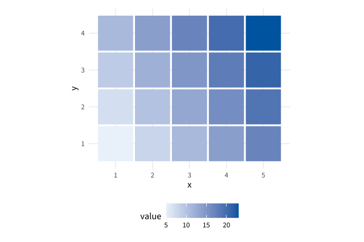
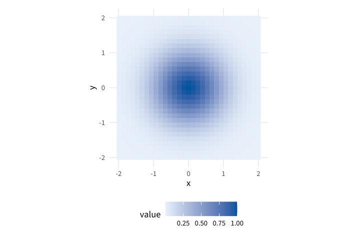
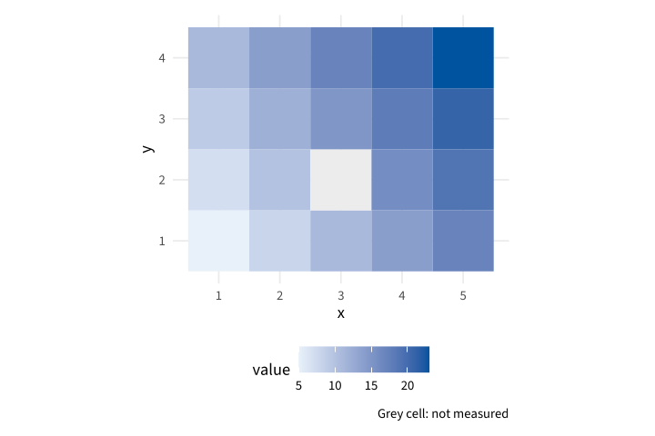
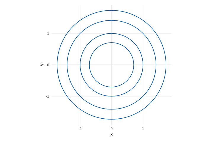
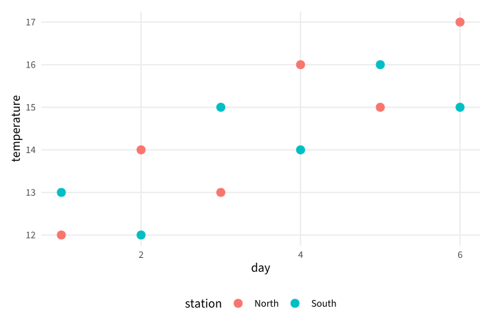
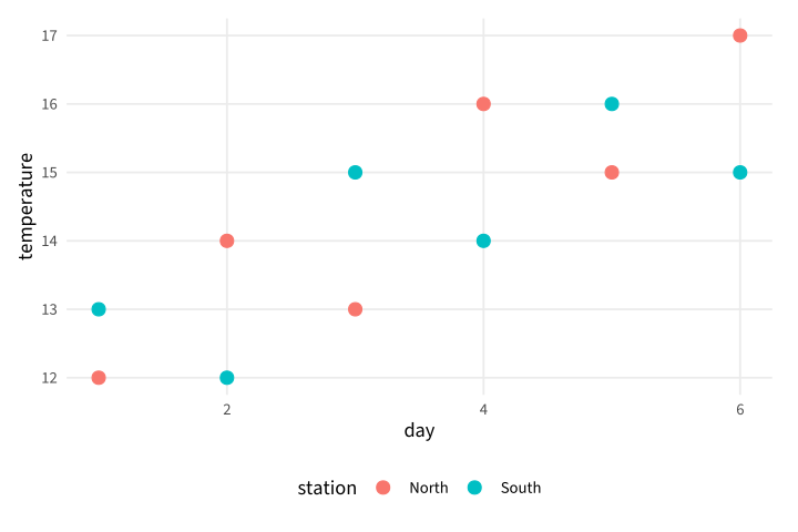
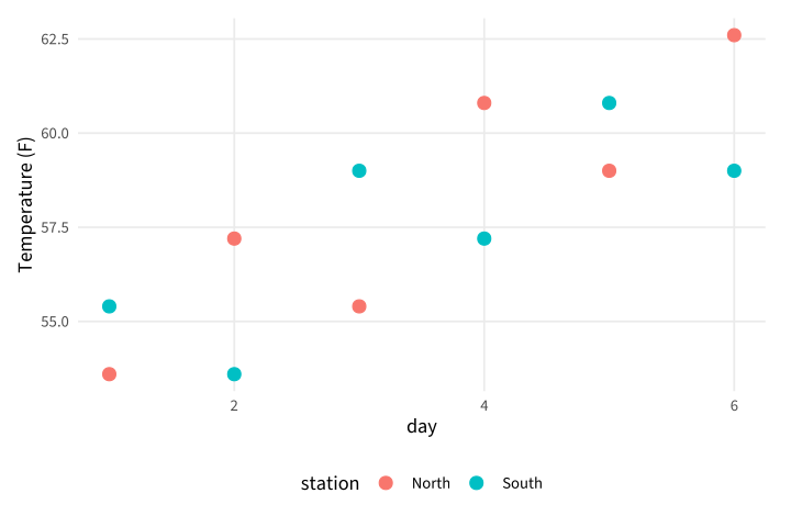
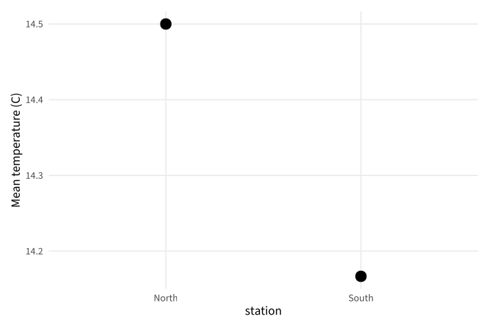
No matching examples. Try another query or clear the filters.
Copy link A visual reference · R / ggplot2
R / ggplot2,
Complete source. One deliberate change. Its actual result.
Follow a small field archive through measurements, distributions and publication graphics. Every chart starts from explicit local data and shows how an aesthetic mapping becomes a native figure.
The Org file is canonical. Read the searchable HTML beside your editor or use the PDF offline. All measurements and operational quantities are synthetic teaching fixtures.
Last changes: 2026-11-16. Original examples, pinned native rendering and portable source/configuration downloads.
96 worked examples
16 topic families
1 canonical Org source
Copy link Reading the tour
Three ways to see a change
Read the source
Each example is a complete file. Identify the syntax introduced before changing it.
Inspect the output
Open a gallery thumbnail, compare the native figure and follow a sibling example.
Make a change
Download the source/configuration ZIP, make the suggested edit and repeat its exact command.
Browse this tour with the gallery, search and topic filters. Stable IDs identify chapters and examples; Back to diagram overview returns to the corresponding thumbnail. The shared configuration sets appearance, never example data.
Copy link Reproduce the diagrams
The reviewed native toolchain is R 4.6.2, ggplot2 4.0.4 and Poppler 26.11.0 . Exact checksums and publisher versions are recorded in VERSIONS.json. Install R 4.6.2, Poppler and a C/C++ compiler. Run python3 tools/install-R once to install the pinned package sources from tools/vendor/ into the ignored .R-library/ directory. This installation reads its local package index and needs no network. The renderer uses the bundled Source Sans 3 font and native Cairo PDF; Poppler creates SVG and PNG companions.
Install the shared publisher with make setup in its sibling directory. Activate that Python environment before using a standalone bundle, or install its pinned requirements.txt in a fresh environment. The published HTML embeds figures and works offline; keep the companion directories for individual downloads.
make full
make check
tools/render --version
tools/render examples/GGP-01-001.R
Command or configuration
Meaning in this tour
tools/render SOURCERun the pinned native pipeline and write PDF, SVG and PNG.
config/render.jsonReviewed tool versions and bundled font checksums.
SOURCE_DATE_EPOCH=0Fix native build-date inputs; the driver removes PDF date metadata.
make fullExplicitly execute reviewed programs, then build HTML and PDF.
makeReuse verified local results; never execute examples implicitly.
make checkVerify output hashes, example IDs and offline links.
Rscript --vanillaEvaluate the complete program without user startup files.
config/style.RSet the common theme, local font, warning policy and six-by-four-inch Cairo PDF export.
config/packages.jsonExact package versions and checksums of bundled source archives.
tools/install-RCompile the reviewed package sources from a local file repository.
pdftocairo -svgConvert the native Cairo PDF to a self-contained SVG companion.
Download the complete reproduction bundle to run all examples, or inspect the shared render configuration . After installing system tools and the shared Python dependencies, preparation and rendering use no network. SVG is self-contained; native PDF pages are placed directly in the guide. Most layers are vector artwork; the raster example deliberately embeds its image layer. Repair sources rather than editing generated figures.
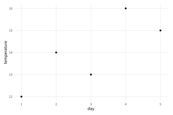
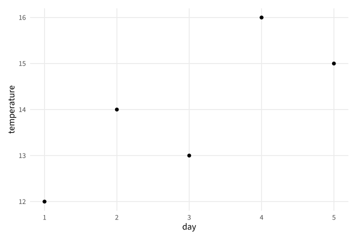
Copy link GGP-01-001 Place the measurements A point layer maps two numeric columns to positions. Use it to inspect paired measurements before adding a trend or statistical model.
Back to diagram overview Compare with gnuplot plotting tour .
Complete R / ggplot2 source source ( "config/style.R" )
d <- data.frame ( day = 1 : 5 , temperature = c ( 12 , 14 , 13 , 16 , 15 ))
p <- ggplot ( d , aes ( day , temperature )) + geom_point ()
export_plot ( p , "GGP-01-001" )
Parameter Meaning in this example aes(day, temperature)Map the two columns to horizontal and vertical positions. geom_point()Draw one point for every observation.
Render this diagram examples/GGP-01-001.R
Try changing: Change the fourth temperature to 18.
Actual output GGP-01-001 · R / ggplot2 native output R / ggplot2 · exit 0
Native compiler log Standard output Download: Source · Source + configuration ZIP · SVG · Native PDF · PNG
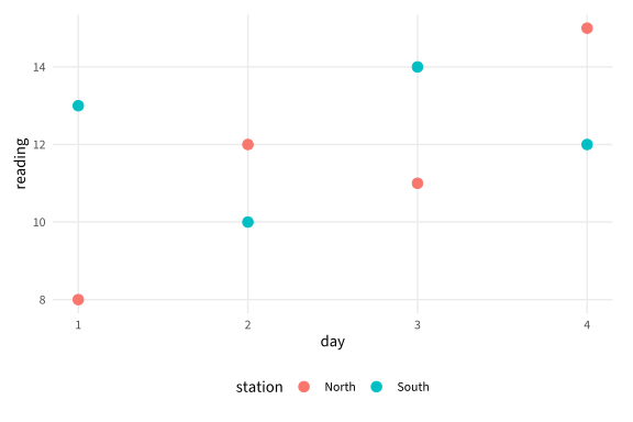
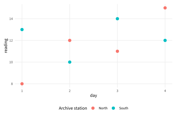
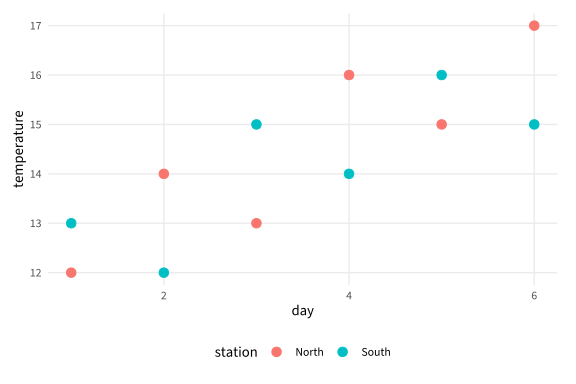
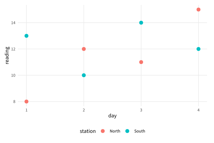
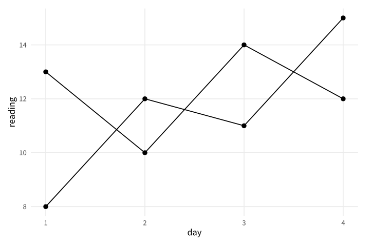
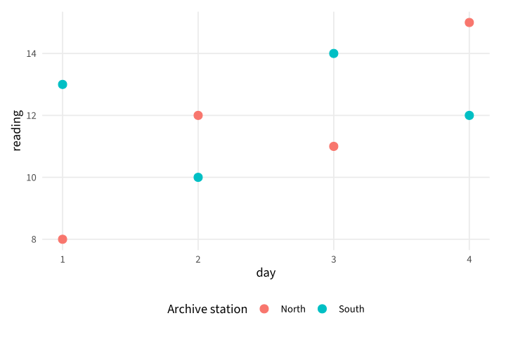
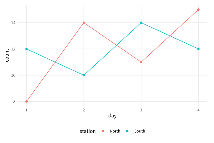
Copy link GGP-01-002 Map a third variable to color An aesthetic mapping can carry a group identity as well as a position. Use a color legend when the field stations need to remain distinguishable.
Back to diagram overview Compare with GGP-01-001 · Place the measurements .
Complete R / ggplot2 source source ( "config/style.R" )
d <- data.frame ( station = rep ( c ( "North" , "South" ), each = 4 ),
day = rep ( 1 : 4 , 2 ), reading = c ( 8 , 12 , 11 , 15 , 13 , 10 , 14 , 12 ))
p <- ggplot ( d , aes ( day , reading , colour = station )) + geom_point ( size = 3 )
export_plot ( p , "GGP-01-002" )
Parameter Meaning in this example colour=stationMap station identity to a color scale and legend.
Render this diagram examples/GGP-01-002.R
Try changing: Rename the two stations.
Actual output GGP-01-002 · R / ggplot2 native output R / ggplot2 · exit 0
Native compiler log Standard output Download: Source · Source + configuration ZIP · SVG · Native PDF · PNG
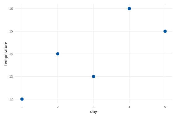
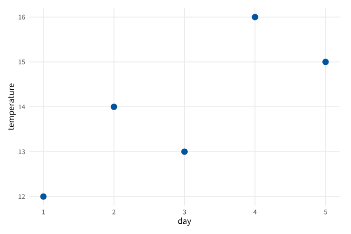
Copy link GGP-01-003 Set a constant appearance A constant outside aes applies to every mark. Use it for a presentation choice that does not represent another data variable.
Back to diagram overview Compare with GGP-01-002 · Map a third variable to color .
Complete R / ggplot2 source source ( "config/style.R" )
d <- data.frame ( day = 1 : 5 , temperature = c ( 12 , 14 , 13 , 16 , 15 ))
p <- ggplot ( d , aes ( day , temperature )) +
geom_point ( colour = "#00549F" , size = 3 )
export_plot ( p , "GGP-01-003" )
Parameter Meaning in this example colour outside aesSet a common color rather than mapping a data field.
Render this diagram examples/GGP-01-003.R
Try changing: Change the fixed color to #C45A18.
Actual output GGP-01-003 · R / ggplot2 native output R / ggplot2 · exit 0
Native compiler log Standard output Download: Source · Source + configuration ZIP · SVG · Native PDF · PNG
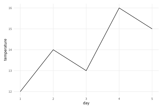
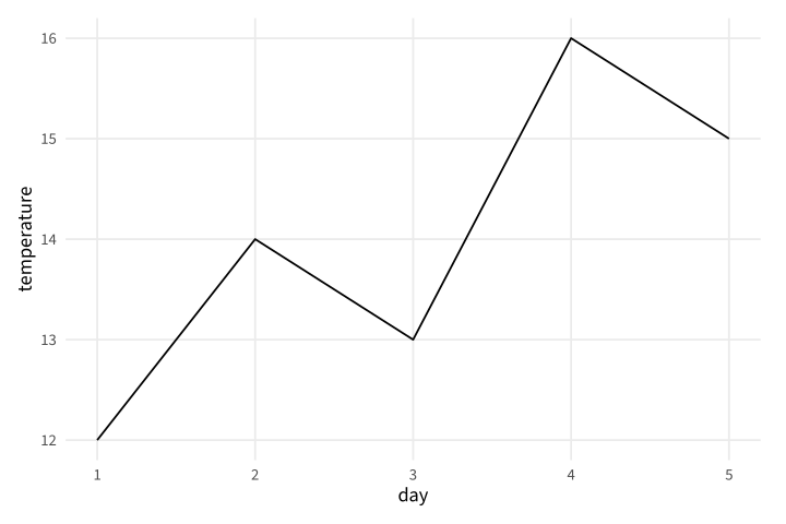
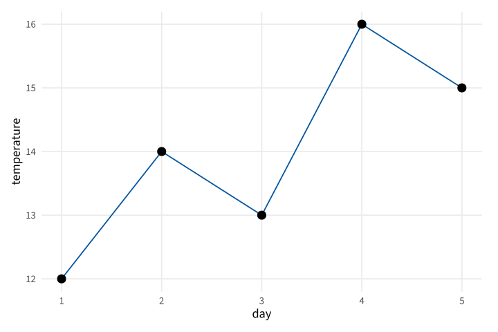
Copy link GGP-01-004 Connect an ordered series A line layer connects values in horizontal order. Use it for readings whose day coordinate defines a meaningful sequence.
Back to diagram overview Compare with GGP-01-003 · Set a constant appearance .
Complete R / ggplot2 source source ( "config/style.R" )
d <- data.frame ( day = 1 : 5 , temperature = c ( 12 , 14 , 13 , 16 , 15 ))
p <- ggplot ( d , aes ( day , temperature )) + geom_line ()
export_plot ( p , "GGP-01-004" )
Parameter Meaning in this example geom_line()Connect the supplied measurements by day.
Render this diagram examples/GGP-01-004.R
Try changing: Move the fourth reading to day 4.5.
Actual output GGP-01-004 · R / ggplot2 native output R / ggplot2 · exit 0
Native compiler log Standard output Download: Source · Source + configuration ZIP · SVG · Native PDF · PNG
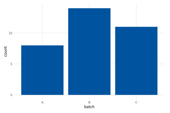
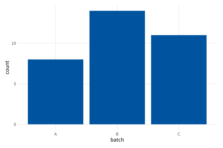
Copy link GGP-01-005 Draw supplied category totals A column layer uses the provided heights directly. Use it when counts have already been calculated rather than asking a plotting layer to count rows.
Back to diagram overview Compare with GGP-01-004 · Connect an ordered series .
Complete R / ggplot2 source source ( "config/style.R" )
d <- data.frame ( batch = c ( "A" , "B" , "C" ), count = c ( 8 , 14 , 11 ))
p <- ggplot ( d , aes ( batch , count )) + geom_col ( fill = "#00549F" )
export_plot ( p , "GGP-01-005" )
Parameter Meaning in this example geom_col()Use supplied totals as bar heights.
Render this diagram examples/GGP-01-005.R
Try changing: Change batch B to 17.
Actual output GGP-01-005 · R / ggplot2 native output R / ggplot2 · exit 0
Native compiler log Standard output Download: Source · Source + configuration ZIP · SVG · Native PDF · PNG
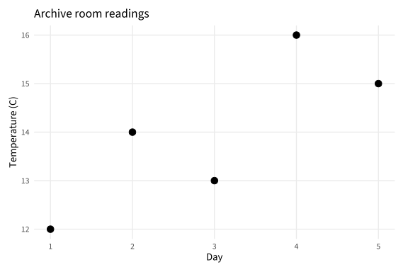
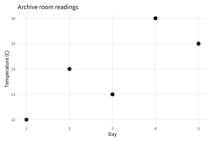
Copy link GGP-01-006 Name the question and units Labels turn mapped columns into a chart that can stand alone. Use a clear title and units instead of leaving readers to infer the measurement.
Back to diagram overview Compare with GGP-01-005 · Draw supplied category totals .
Complete R / ggplot2 source source ( "config/style.R" )
d <- data.frame ( day = 1 : 5 , temperature = c ( 12 , 14 , 13 , 16 , 15 ))
p <- ggplot ( d , aes ( day , temperature )) + geom_point ( size = 3 ) +
labs ( title = "Archive room readings" , x = "Day" , y = "Temperature (C)" )
export_plot ( p , "GGP-01-006" )
Parameter Meaning in this example labs()Set the title and human-readable axis labels.
Render this diagram examples/GGP-01-006.R
Try changing: Change the title to identify a different room.
Actual output GGP-01-006 · R / ggplot2 native output R / ggplot2 · exit 0
Native compiler log Standard output Download: Source · Source + configuration ZIP · SVG · Native PDF · PNG
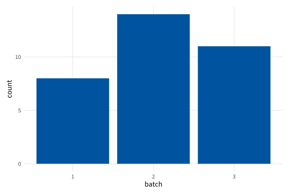
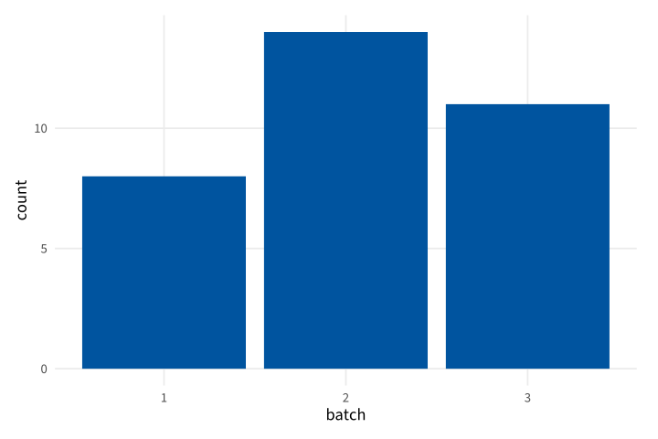
Copy link GGP-02-001 Treat a code as a category A factor tells the scale that values are category codes. Use it when numbers identify batches rather than measured distances.
Back to diagram overview Compare with GGP-01-005 · Draw supplied category totals .
Complete R / ggplot2 source source ( "config/style.R" )
d <- data.frame ( batch = factor ( c ( 1 , 2 , 3 )), count = c ( 8 , 14 , 11 ))
p <- ggplot ( d , aes ( batch , count )) + geom_col ( fill = "#00549F" )
export_plot ( p , "GGP-02-001" )
Parameter Meaning in this example factor()Represent batch identifiers as discrete categories.
Render this diagram examples/GGP-02-001.R
Try changing: Replace the levels with A, B and C.
Actual output GGP-02-001 · R / ggplot2 native output R / ggplot2 · exit 0
Native compiler log Standard output Download: Source · Source + configuration ZIP · SVG · Native PDF · PNG
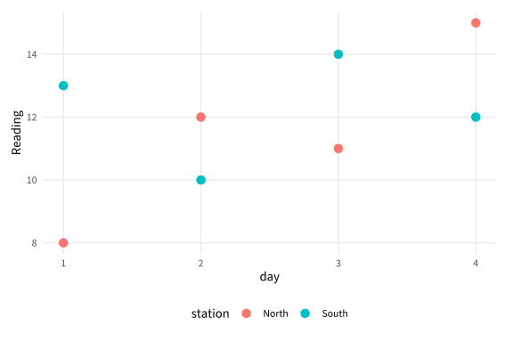
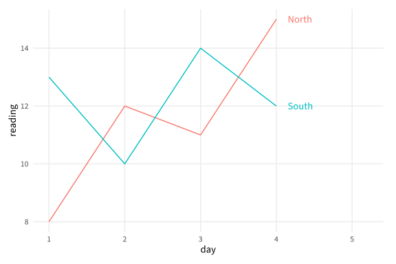
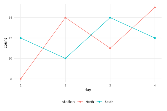
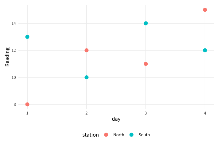
Copy link GGP-02-002 Keep series in a long table A long table stores one measured value per row and a group column. Use this structure when multiple stations share the same plotting rule.
Back to diagram overview Compare with GGP-02-001 · Treat a code as a category .
Complete R / ggplot2 source source ( "config/style.R" )
d <- data.frame ( station = rep ( c ( "North" , "South" ), each = 4 ),
day = rep ( 1 : 4 , 2 ), reading = c ( 8 , 12 , 11 , 15 , 13 , 10 , 14 , 12 ))
p <- ggplot ( d , aes ( day , reading , colour = station )) +
geom_point ( size = 3 ) + labs ( y = "Reading" )
export_plot ( p , "GGP-02-002" )
Parameter Meaning in this example One value columnKeep all readings in one column and identify their station separately.
Render this diagram examples/GGP-02-002.R
Try changing: Add a third station with four observations.
Actual output GGP-02-002 · R / ggplot2 native output R / ggplot2 · exit 0
Native compiler log Standard output Download: Source · Source + configuration ZIP · SVG · Native PDF · PNG
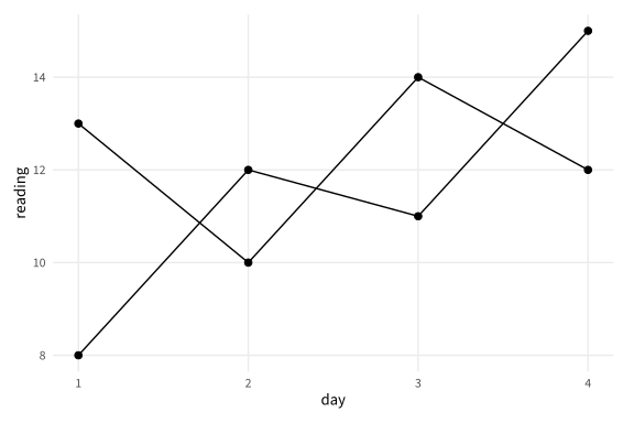
Copy link GGP-02-003 Group connections explicitly A group mapping says which observations belong to the same line. Use it when a continuous color or shared appearance would not establish the intended grouping.
Back to diagram overview Compare with GGP-02-002 · Keep series in a long table .
Complete R / ggplot2 source source ( "config/style.R" )
d <- data.frame ( station = rep ( c ( "North" , "South" ), each = 4 ),
day = rep ( 1 : 4 , 2 ), reading = c ( 8 , 12 , 11 , 15 , 13 , 10 , 14 , 12 ))
p <- ggplot ( d , aes ( day , reading , group = station )) +
geom_line () + geom_point ( size = 2 )
export_plot ( p , "GGP-02-003" )
Parameter Meaning in this example group=stationKeep each station's line independent.
Render this diagram examples/GGP-02-003.R
Try changing: Remove group temporarily and inspect the connections.
Actual output GGP-02-003 · R / ggplot2 native output R / ggplot2 · exit 0
Native compiler log Standard output Download: Source · Source + configuration ZIP · SVG · Native PDF · PNG
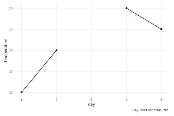
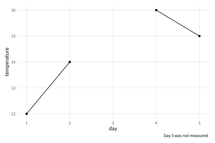
Copy link GGP-02-004 Keep a visible gap for missing data An NA represents an unavailable measurement rather than zero. Keep it in the sequence so the line does not imply an observed connection across the gap.
Back to diagram overview Compare with GGP-02-003 · Group connections explicitly .
Complete R / ggplot2 source source ( "config/style.R" )
d <- data.frame ( day = 1 : 5 , temperature = c ( 12 , 14 , NA , 16 , 15 ))
p <- ggplot ( d , aes ( day , temperature )) +
geom_line ( na.rm = TRUE ) + geom_point ( na.rm = TRUE ) +
labs ( caption = "Day 3 was not measured" )
export_plot ( p , "GGP-02-004" )
Parameter Meaning in this example NAMark the unavailable reading explicitly. na.rm=TRUEOmit missing marks while preserving the supplied gap in the line.
Render this diagram examples/GGP-02-004.R
Try changing: Replace the missing value with 13 and update the caption.
Actual output GGP-02-004 · R / ggplot2 native output R / ggplot2 · exit 0
Native compiler log Standard output Download: Source · Source + configuration ZIP · SVG · Native PDF · PNG
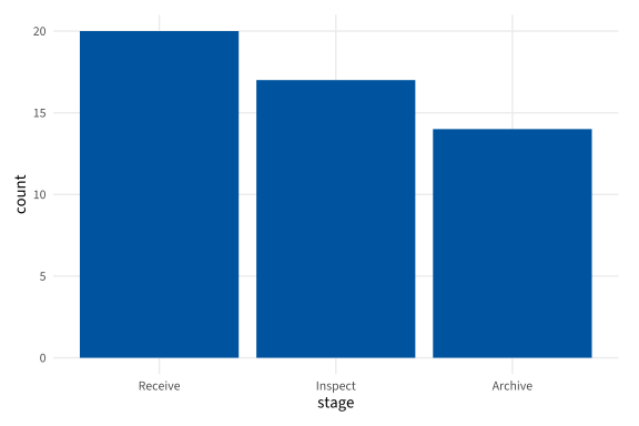
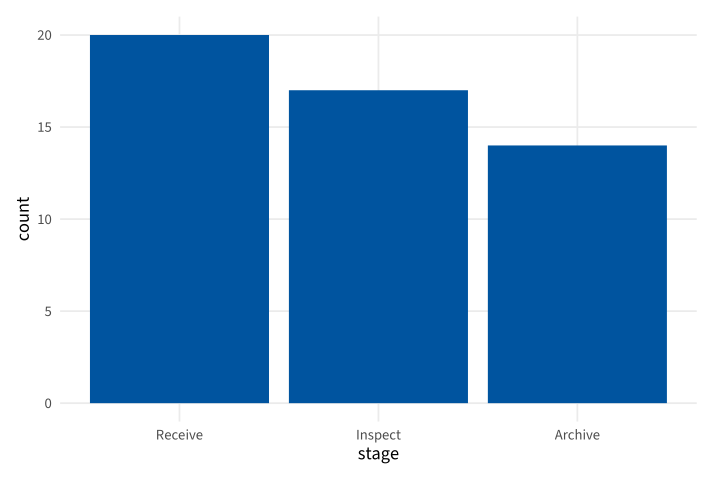
Copy link GGP-02-005 Order categories deliberately Explicit factor levels control the display order. Use a process or reporting order instead of inheriting alphabetical sorting.
Back to diagram overview Compare with GGP-02-004 · Keep a visible gap for missing data .
Complete R / ggplot2 source source ( "config/style.R" )
d <- data.frame ( stage = c ( "Receive" , "Inspect" , "Archive" ), count = c ( 20 , 17 , 14 ))
d $ stage <- factor ( d $ stage , levels = c ( "Receive" , "Inspect" , "Archive" ))
p <- ggplot ( d , aes ( stage , count )) + geom_col ( fill = "#00549F" )
export_plot ( p , "GGP-02-005" )
Parameter Meaning in this example levels=Set the intended left-to-right category order.
Render this diagram examples/GGP-02-005.R
Try changing: Reverse the level order.
Actual output GGP-02-005 · R / ggplot2 native output R / ggplot2 · exit 0
Native compiler log Standard output Download: Source · Source + configuration ZIP · SVG · Native PDF · PNG
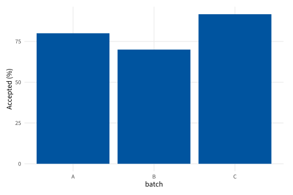
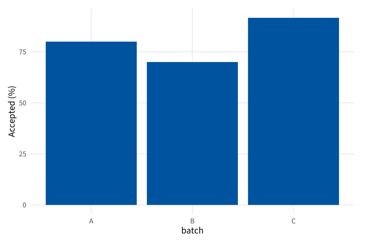
Copy link GGP-02-006 Calculate a displayed rate A derived column makes a ratio and its denominator visible in the source. Use explicit denominators when groups have different totals.
Back to diagram overview Compare with GGP-02-005 · Order categories deliberately .
Complete R / ggplot2 source source ( "config/style.R" )
d <- data.frame ( batch = c ( "A" , "B" , "C" ), accepted = c ( 8 , 14 , 11 ), total = c ( 10 , 20 , 12 ))
d $ percent <- 100 * d $ accepted / d $ total
p <- ggplot ( d , aes ( batch , percent )) + geom_col ( fill = "#00549F" ) +
labs ( y = "Accepted (%)" )
export_plot ( p , "GGP-02-006" )
Parameter Meaning in this example accepted / totalCalculate each batch rate with its own denominator.
Render this diagram examples/GGP-02-006.R
Try changing: Change batch B total to 25.
Actual output GGP-02-006 · R / ggplot2 native output R / ggplot2 · exit 0
Native compiler log Standard output Download: Source · Source + configuration ZIP · SVG · Native PDF · PNG
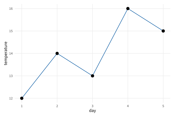
Copy link GGP-03-001 Show samples on their trend Points identify the observed sampling positions on a connected series. Use both layers when readers should distinguish measurements from the line between them.
Back to diagram overview Compare with GGP-01-004 · Connect an ordered series .
Complete R / ggplot2 source source ( "config/style.R" )
d <- data.frame ( day = 1 : 5 , temperature = c ( 12 , 14 , 13 , 16 , 15 ))
p <- ggplot ( d , aes ( day , temperature )) +
geom_line ( colour = "#00549F" ) + geom_point ( size = 3 )
export_plot ( p , "GGP-03-001" )
Parameter Meaning in this example Layer additionDraw the line first and the observed points above it.
Render this diagram examples/GGP-03-001.R
Try changing: Increase only the point size to 4.
Actual output GGP-03-001 · R / ggplot2 native output R / ggplot2 · exit 0
Native compiler log Standard output Download: Source · Source + configuration ZIP · SVG · Native PDF · PNG
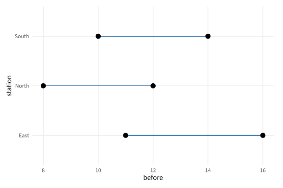
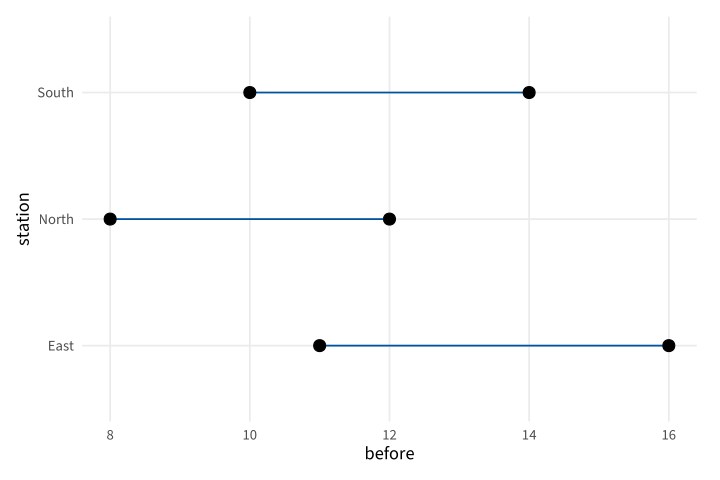
Copy link GGP-03-002 Connect paired values with segments A segment has explicit start and end coordinates. Use it to compare two supplied readings for the same station.
Back to diagram overview Compare with GGP-03-001 · Show samples on their trend .
Complete R / ggplot2 source source ( "config/style.R" )
d <- data.frame ( station = c ( "North" , "South" , "East" ), before = c ( 8 , 14 , 11 ), after = c ( 12 , 10 , 16 ))
p <- ggplot ( d , aes ( y = station )) +
geom_segment ( aes ( x = before , xend = after , yend = station ), colour = "#00549F" ) +
geom_point ( aes ( x = before ), size = 3 ) + geom_point ( aes ( x = after ), size = 3 )
export_plot ( p , "GGP-03-002" )
Parameter Meaning in this example xend / yendSpecify the other endpoint of each paired comparison.
Render this diagram examples/GGP-03-002.R
Try changing: Change the East after value to 13.
Actual output GGP-03-002 · R / ggplot2 native output R / ggplot2 · exit 0
Native compiler log Standard output Download: Source · Source + configuration ZIP · SVG · Native PDF · PNG
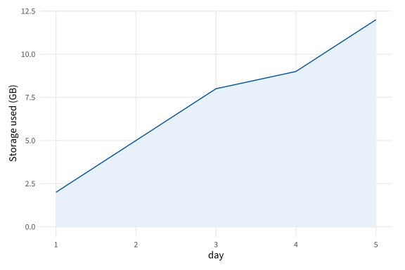
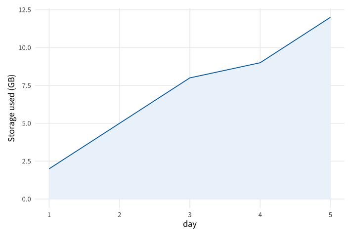
Copy link GGP-03-003 Fill the area under a supplied series An area layer relates a height to its baseline. Use it for an ordered quantity whose filled extent has a stated meaning, such as cumulative storage use.
Back to diagram overview Compare with GGP-03-002 · Connect paired values with segments .
Complete R / ggplot2 source source ( "config/style.R" )
d <- data.frame ( day = 1 : 5 , used = c ( 2 , 5 , 8 , 9 , 12 ))
p <- ggplot ( d , aes ( day , used )) + geom_area ( fill = "#E8F1FA" , colour = "#00549F" ) +
labs ( y = "Storage used (GB)" )
export_plot ( p , "GGP-03-003" )
Parameter Meaning in this example geom_area()Fill between the ordered series and zero.
Render this diagram examples/GGP-03-003.R
Try changing: Change the last value to 15.
Actual output GGP-03-003 · R / ggplot2 native output R / ggplot2 · exit 0
Native compiler log Standard output Download: Source · Source + configuration ZIP · SVG · Native PDF · PNG
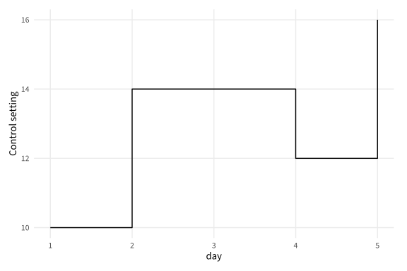
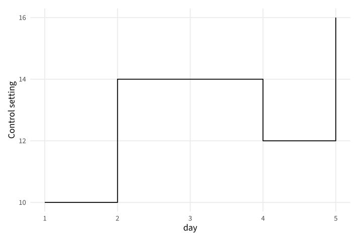
Copy link GGP-03-004 Draw a stepwise state A step layer holds a value until the next supplied change. Use it for settings or recorded state changes rather than smoothly varying measurements.
Back to diagram overview Compare with GGP-03-003 · Fill the area under a supplied series .
Complete R / ggplot2 source source ( "config/style.R" )
d <- data.frame ( day = c ( 1 , 2 , 4 , 5 ), setting = c ( 10 , 14 , 12 , 16 ))
p <- ggplot ( d , aes ( day , setting )) + geom_step ( direction = "hv" ) +
labs ( y = "Control setting" )
export_plot ( p , "GGP-03-004" )
Parameter Meaning in this example direction="hv"Travel horizontally before the vertical change.
Render this diagram examples/GGP-03-004.R
Try changing: Change direction to vh and compare when each jump occurs.
Actual output GGP-03-004 · R / ggplot2 native output R / ggplot2 · exit 0
Native compiler log Standard output Download: Source · Source + configuration ZIP · SVG · Native PDF · PNG
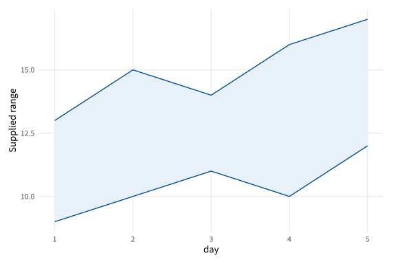
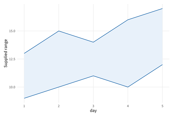
Copy link GGP-03-005 Show a supplied range as a band A ribbon draws explicit lower and upper bounds. Use it when a range is known independently of a plotting layer's statistical estimator.
Back to diagram overview Compare with GGP-03-004 · Draw a stepwise state .
Complete R / ggplot2 source source ( "config/style.R" )
d <- data.frame ( day = 1 : 5 , low = c ( 9 , 10 , 11 , 10 , 12 ), high = c ( 13 , 15 , 14 , 16 , 17 ))
p <- ggplot ( d , aes ( day )) +
geom_ribbon ( aes ( ymin = low , ymax = high ), fill = "#E8F1FA" , colour = "#00549F" ) +
labs ( y = "Supplied range" )
export_plot ( p , "GGP-03-005" )
Parameter Meaning in this example ymin / ymaxProvide the two boundaries of the range band.
Render this diagram examples/GGP-03-005.R
Try changing: Increase the fourth upper bound to 18.
Actual output GGP-03-005 · R / ggplot2 native output R / ggplot2 · exit 0
Native compiler log Standard output Download: Source · Source + configuration ZIP · SVG · Native PDF · PNG
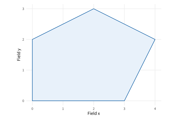
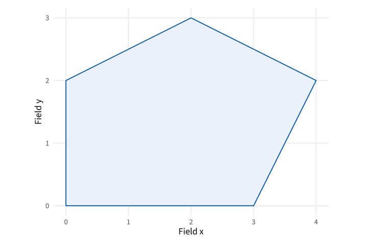
Copy link GGP-03-006 Close an explicit polygon A polygon joins ordered vertices and closes the boundary. Use it for a supplied region such as a simplified field enclosure.
Back to diagram overview Compare with GGP-03-005 · Show a supplied range as a band .
Complete R / ggplot2 source source ( "config/style.R" )
d <- data.frame ( x = c ( 0 , 3 , 4 , 2 , 0 ), y = c ( 0 , 0 , 2 , 3 , 2 ))
p <- ggplot ( d , aes ( x , y )) + geom_polygon ( fill = "#E8F1FA" , colour = "#00549F" ) +
coord_equal () + labs ( x = "Field x" , y = "Field y" )
export_plot ( p , "GGP-03-006" )
Parameter Meaning in this example geom_polygon()Join the supplied vertices and close the region.
Render this diagram examples/GGP-03-006.R
Try changing: Move the top vertex from y=3 to y=4.
Actual output GGP-03-006 · R / ggplot2 native output R / ggplot2 · exit 0
Native compiler log Standard output Download: Source · Source + configuration ZIP · SVG · Native PDF · PNG
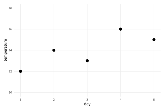
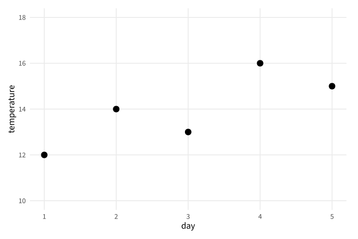
Copy link GGP-04-001 Choose readable axis breaks Explicit breaks make the reading intervals consistent. Use them when a set of related charts should share a familiar scale.
Back to diagram overview Compare with GGP-01-001 · Place the measurements .
Complete R / ggplot2 source source ( "config/style.R" )
d <- data.frame ( day = 1 : 5 , temperature = c ( 12 , 14 , 13 , 16 , 15 ))
p <- ggplot ( d , aes ( day , temperature )) + geom_point ( size = 3 ) +
scale_y_continuous ( breaks = seq ( 10 , 18 , 2 ), limits = c ( 10 , 18 ))
export_plot ( p , "GGP-04-001" )
Parameter Meaning in this example breaks / limitsSpecify displayed tick values and the complete scale domain.
Render this diagram examples/GGP-04-001.R
Try changing: Change the interval to one degree.
Actual output GGP-04-001 · R / ggplot2 native output R / ggplot2 · exit 0
Native compiler log Standard output Download: Source · Source + configuration ZIP · SVG · Native PDF · PNG
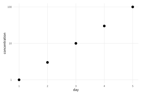
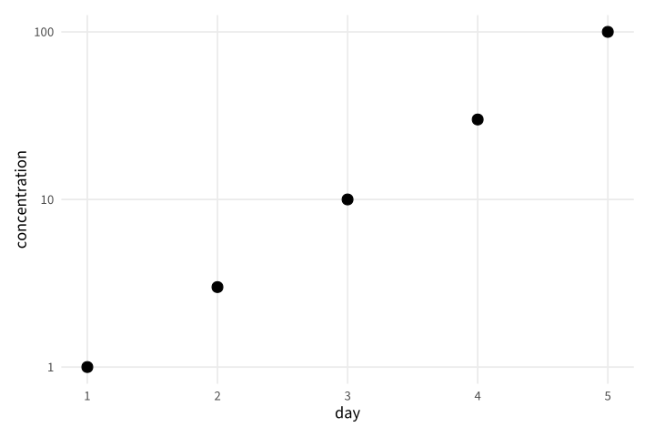
Copy link GGP-04-002 Plot multiplicative values logarithmically A log scale gives equal distance to equal ratios. Use it for strictly positive readings that span orders of magnitude.
Back to diagram overview Compare with GGP-04-001 · Choose readable axis breaks .
Complete R / ggplot2 source source ( "config/style.R" )
d <- data.frame ( day = 1 : 5 , concentration = c ( 1 , 3 , 10 , 30 , 100 ))
p <- ggplot ( d , aes ( day , concentration )) + geom_point ( size = 3 ) + scale_y_log10 ()
export_plot ( p , "GGP-04-002" )
Parameter Meaning in this example scale_y_log10()Map positive values using base-ten logarithms.
Render this diagram examples/GGP-04-002.R
Try changing: Change the final concentration to 300.
Actual output GGP-04-002 · R / ggplot2 native output R / ggplot2 · exit 0
Native compiler log Standard output Download: Source · Source + configuration ZIP · SVG · Native PDF · PNG
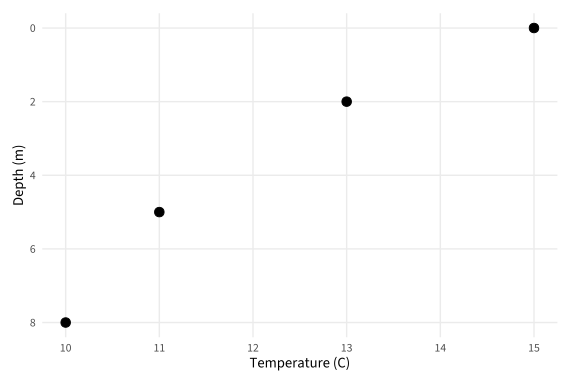
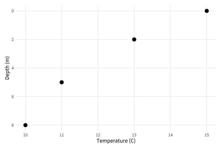
Copy link GGP-04-003 Reverse a depth axis A reversed scale can make increasing depth run downward. Use a unit label so the direction has a clear physical interpretation.
Back to diagram overview Compare with GGP-04-002 · Plot multiplicative values logarithmically .
Complete R / ggplot2 source source ( "config/style.R" )
d <- data.frame ( temperature = c ( 15 , 13 , 11 , 10 ), depth = c ( 0 , 2 , 5 , 8 ))
p <- ggplot ( d , aes ( temperature , depth )) + geom_point ( size = 3 ) +
scale_y_reverse () + labs ( y = "Depth (m)" , x = "Temperature (C)" )
export_plot ( p , "GGP-04-003" )
Parameter Meaning in this example scale_y_reverse()Place larger depth values lower in the plot.
Render this diagram examples/GGP-04-003.R
Try changing: Add a reading at depth 10.
Actual output GGP-04-003 · R / ggplot2 native output R / ggplot2 · exit 0
Native compiler log Standard output Download: Source · Source + configuration ZIP · SVG · Native PDF · PNG
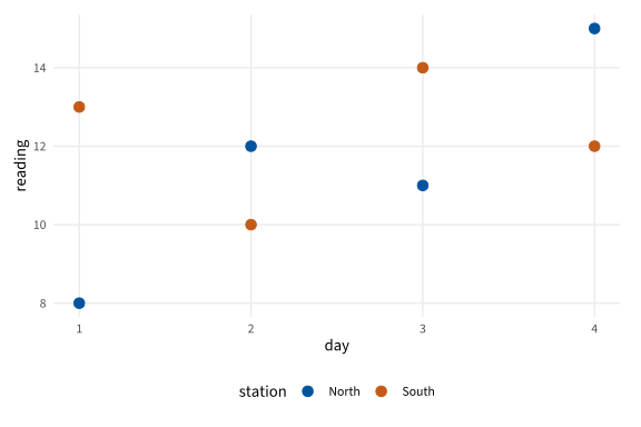
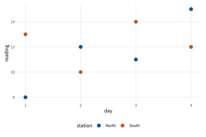
Copy link GGP-04-004 Assign stable group colors A named manual scale keeps a group color stable when row order changes. Use this when the same station appears in multiple figures.
Back to diagram overview Compare with GGP-04-003 · Reverse a depth axis .
Complete R / ggplot2 source source ( "config/style.R" )
d <- data.frame ( station = rep ( c ( "North" , "South" ), each = 4 ),
day = rep ( 1 : 4 , 2 ), reading = c ( 8 , 12 , 11 , 15 , 13 , 10 , 14 , 12 ))
p <- ggplot ( d , aes ( day , reading , colour = station )) + geom_point ( size = 3 ) +
scale_colour_manual ( values = c ( North = "#00549F" , South = "#C45A18" ))
export_plot ( p , "GGP-04-004" )
Parameter Meaning in this example Named color valuesAssociate each color with its station name.
Render this diagram examples/GGP-04-004.R
Try changing: Swap the two named colors.
Actual output GGP-04-004 · R / ggplot2 native output R / ggplot2 · exit 0
Native compiler log Standard output Download: Source · Source + configuration ZIP · SVG · Native PDF · PNG
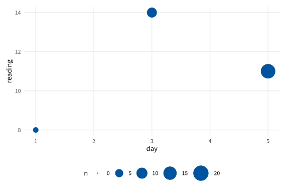
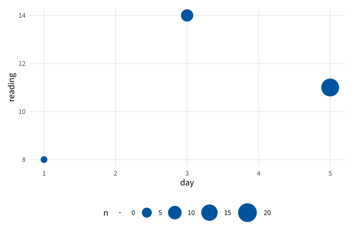
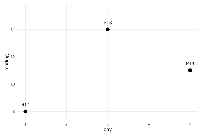
Copy link GGP-04-005 Scale circle area to sample size An area scale makes a larger marker represent more observations. Include zero in the scale definition so an empty count has zero area.
Back to diagram overview Compare with GGP-04-004 · Assign stable group colors .
Complete R / ggplot2 source source ( "config/style.R" )
d <- data.frame ( day = c ( 1 , 3 , 5 ), reading = c ( 8 , 14 , 11 ), n = c ( 2 , 8 , 18 ))
p <- ggplot ( d , aes ( day , reading , size = n )) + geom_point ( colour = "#00549F" ) +
scale_size_area ( max_size = 10 , limits = c ( 0 , 20 ))
export_plot ( p , "GGP-04-005" )
Parameter Meaning in this example scale_size_area()Map count to marker area with a zero-sized origin.
Render this diagram examples/GGP-04-005.R
Try changing: Change the middle count to 12.
Actual output GGP-04-005 · R / ggplot2 native output R / ggplot2 · exit 0
Native compiler log Standard output Download: Source · Source + configuration ZIP · SVG · Native PDF · PNG
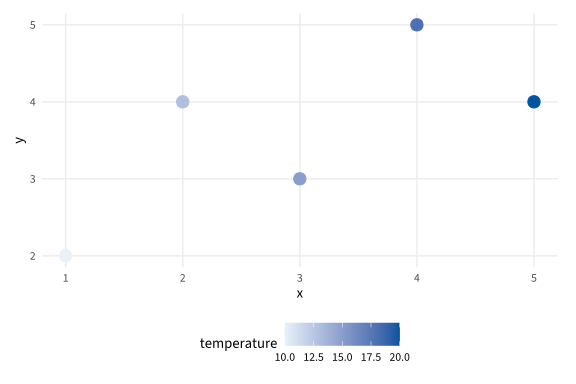
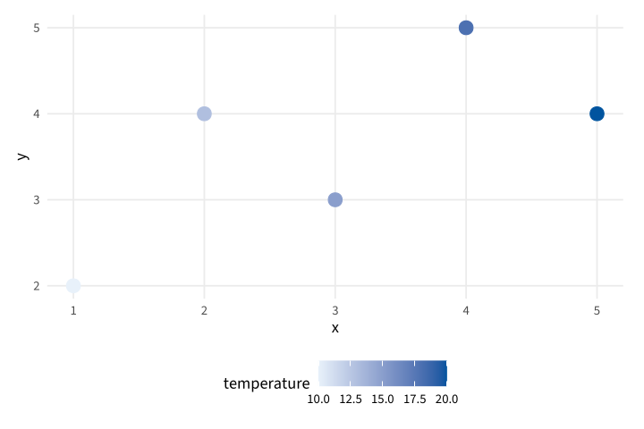
Copy link GGP-04-006 Map a measured value continuously A continuous color scale represents a numeric field. Use a fixed range when the same colors must mean the same values in another chart.
Back to diagram overview Compare with GGP-04-005 · Scale circle area to sample size .
Complete R / ggplot2 source source ( "config/style.R" )
d <- data.frame ( x = 1 : 5 , y = c ( 2 , 4 , 3 , 5 , 4 ), temperature = c ( 10 , 13 , 15 , 18 , 20 ))
p <- ggplot ( d , aes ( x , y , colour = temperature )) + geom_point ( size = 4 ) +
scale_colour_gradient ( low = "#E8F1FA" , high = "#00549F" , limits = c ( 10 , 20 ))
export_plot ( p , "GGP-04-006" )
Parameter Meaning in this example limits=c(10,20)Fix the numeric meaning of the color endpoints.
Render this diagram examples/GGP-04-006.R
Try changing: Change the fixed domain to 5 through 25.
Actual output GGP-04-006 · R / ggplot2 native output R / ggplot2 · exit 0
Native compiler log Standard output Download: Source · Source + configuration ZIP · SVG · Native PDF · PNG
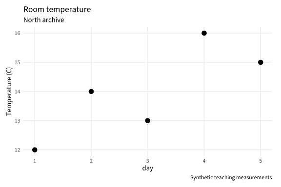
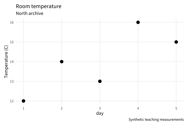
Copy link GGP-05-001 Explain the figure in its caption A subtitle and caption can state scope without crowding the axes. Use them for the archive room and the status of the supplied observations.
Back to diagram overview Compare with GGP-01-006 · Name the question and units .
Complete R / ggplot2 source source ( "config/style.R" )
d <- data.frame ( day = 1 : 5 , temperature = c ( 12 , 14 , 13 , 16 , 15 ))
p <- ggplot ( d , aes ( day , temperature )) + geom_point ( size = 3 ) +
labs ( title = "Room temperature" , subtitle = "North archive" ,
caption = "Synthetic teaching measurements" , y = "Temperature (C)" )
export_plot ( p , "GGP-05-001" )
Parameter Meaning in this example subtitle / captionSeparate the scope from the data and provenance note.
Render this diagram examples/GGP-05-001.R
Try changing: Change the room named in the subtitle.
Actual output GGP-05-001 · R / ggplot2 native output R / ggplot2 · exit 0
Native compiler log Standard output Download: Source · Source + configuration ZIP · SVG · Native PDF · PNG
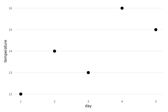
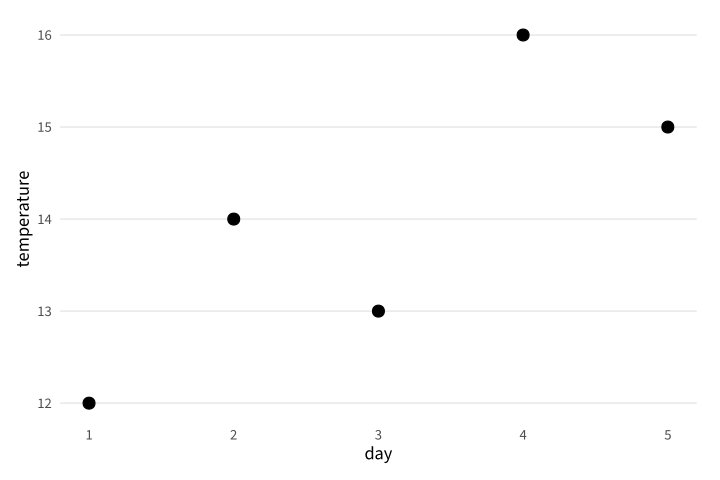
Copy link GGP-05-002 Remove an unhelpful grid direction A theme element can reduce background detail without changing the mapping. Use it when horizontal references suffice for reading the values.
Back to diagram overview Compare with GGP-05-001 · Explain the figure in its caption .
Complete R / ggplot2 source source ( "config/style.R" )
d <- data.frame ( day = 1 : 5 , temperature = c ( 12 , 14 , 13 , 16 , 15 ))
p <- ggplot ( d , aes ( day , temperature )) + geom_point ( size = 3 ) +
theme ( panel.grid.major.x = element_blank ())
export_plot ( p , "GGP-05-002" )
Parameter Meaning in this example element_blank()Omit the selected theme element.
Render this diagram examples/GGP-05-002.R
Try changing: Remove the horizontal grid instead.
Actual output GGP-05-002 · R / ggplot2 native output R / ggplot2 · exit 0
Native compiler log Standard output Download: Source · Source + configuration ZIP · SVG · Native PDF · PNG
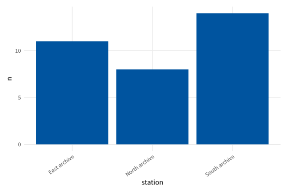
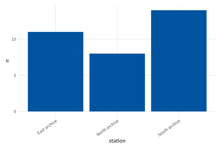
Copy link GGP-05-003 Rotate long category labels A text angle makes long names fit while retaining their full wording. Use the justification to keep the rotated text attached to its tick.
Back to diagram overview Compare with GGP-05-002 · Remove an unhelpful grid direction .
Complete R / ggplot2 source source ( "config/style.R" )
d <- data.frame ( station = c ( "North archive" , "South archive" , "East archive" ), n = c ( 8 , 14 , 11 ))
p <- ggplot ( d , aes ( station , n )) + geom_col ( fill = "#00549F" ) +
theme ( axis.text.x = element_text ( angle = 35 , hjust = 1 ))
export_plot ( p , "GGP-05-003" )
Parameter Meaning in this example angle / hjustRotate category text and align its end with the tick.
Render this diagram examples/GGP-05-003.R
Try changing: Change the angle to 50 degrees.
Actual output GGP-05-003 · R / ggplot2 native output R / ggplot2 · exit 0
Native compiler log Standard output Download: Source · Source + configuration ZIP · SVG · Native PDF · PNG
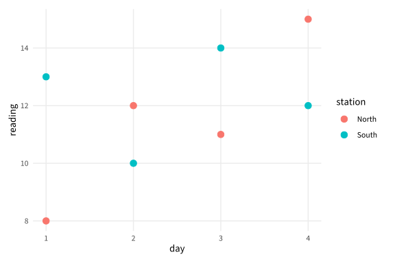
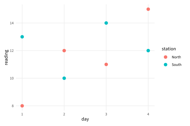
Copy link GGP-05-004 Move a group legend A legend can occupy a side instead of the common lower position. Use this when the panel needs horizontal space for a long time axis.
Back to diagram overview Compare with GGP-05-003 · Rotate long category labels .
Complete R / ggplot2 source source ( "config/style.R" )
d <- data.frame ( station = rep ( c ( "North" , "South" ), each = 4 ),
day = rep ( 1 : 4 , 2 ), reading = c ( 8 , 12 , 11 , 15 , 13 , 10 , 14 , 12 ))
p <- ggplot ( d , aes ( day , reading , colour = station )) + geom_point ( size = 3 ) +
theme ( legend.position = "right" )
export_plot ( p , "GGP-05-004" )
Parameter Meaning in this example legend.positionChoose where the mapped group legend appears.
Render this diagram examples/GGP-05-004.R
Try changing: Move the legend to the top.
Actual output GGP-05-004 · R / ggplot2 native output R / ggplot2 · exit 0
Native compiler log Standard output Download: Source · Source + configuration ZIP · SVG · Native PDF · PNG
Copy link GGP-05-005 Name a legend independently The legend title should explain the field in ordinary language. Use labs to rename it without changing the source column.
Back to diagram overview Compare with GGP-05-004 · Move a group legend .
Complete R / ggplot2 source source ( "config/style.R" )
d <- data.frame ( station = rep ( c ( "North" , "South" ), each = 4 ),
day = rep ( 1 : 4 , 2 ), reading = c ( 8 , 12 , 11 , 15 , 13 , 10 , 14 , 12 ))
p <- ggplot ( d , aes ( day , reading , colour = station )) + geom_point ( size = 3 ) +
labs ( colour = "Archive station" )
export_plot ( p , "GGP-05-005" )
Parameter Meaning in this example labs(colour=)Set the title of the color legend.
Render this diagram examples/GGP-05-005.R
Try changing: Rename the legend to Measurement site.
Actual output GGP-05-005 · R / ggplot2 native output R / ggplot2 · exit 0
Native compiler log Standard output Download: Source · Source + configuration ZIP · SVG · Native PDF · PNG
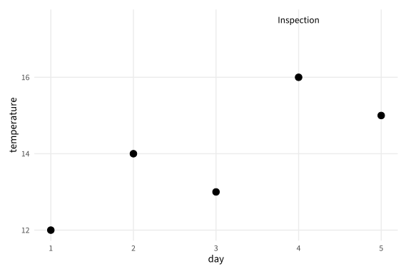
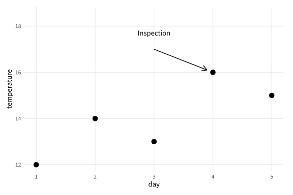
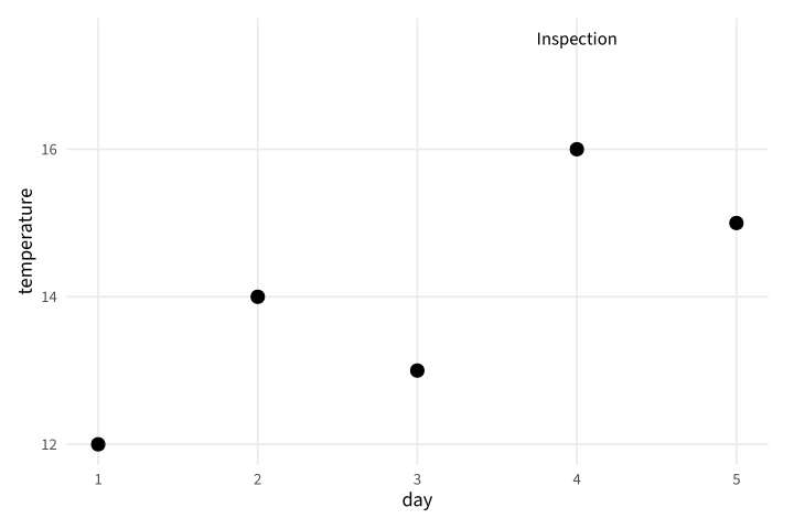
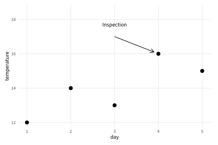
Copy link GGP-05-006 Annotate a specific position An annotation adds explanatory text without creating a new data group. Use explicit coordinates when the note belongs to one supplied event.
Back to diagram overview Compare with GGP-05-005 · Name a legend independently .
Complete R / ggplot2 source source ( "config/style.R" )
d <- data.frame ( day = 1 : 5 , temperature = c ( 12 , 14 , 13 , 16 , 15 ))
p <- ggplot ( d , aes ( day , temperature )) + geom_point ( size = 3 ) +
annotate ( "text" , x = 4 , y = 17.5 , label = "Inspection" , size = 3.5 )
export_plot ( p , "GGP-05-006" )
Parameter Meaning in this example annotate()Add one explanatory label at fixed data coordinates.
Render this diagram examples/GGP-05-006.R
Try changing: Move the note to day 2.
Actual output GGP-05-006 · R / ggplot2 native output R / ggplot2 · exit 0
Native compiler log Standard output Download: Source · Source + configuration ZIP · SVG · Native PDF · PNG
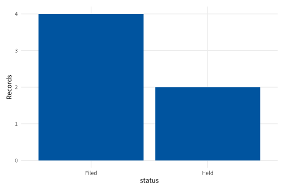
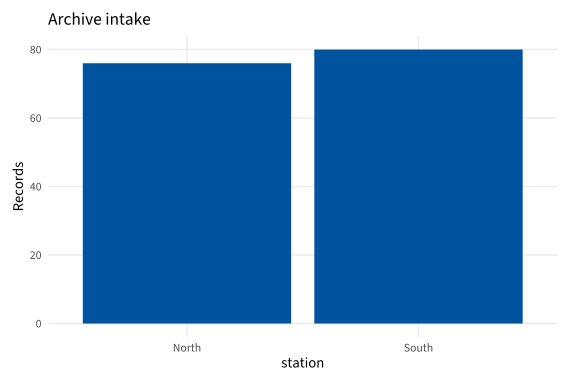
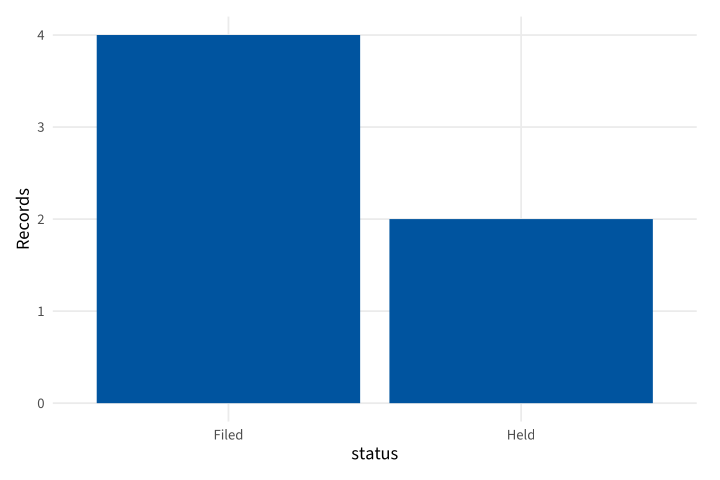
Copy link GGP-06-001 Count the input rows A bar layer can count category occurrences directly. Use it when every input row is one archive record rather than a supplied total.
Back to diagram overview Compare with GGP-01-005 · Draw supplied category totals .
Complete R / ggplot2 source source ( "config/style.R" )
d <- data.frame ( status = c ( "Filed" , "Held" , "Filed" , "Filed" , "Held" , "Filed" ))
p <- ggplot ( d , aes ( status )) + geom_bar ( fill = "#00549F" ) + labs ( y = "Records" )
export_plot ( p , "GGP-06-001" )
Parameter Meaning in this example geom_bar()Count rows in each category.
Render this diagram examples/GGP-06-001.R
Try changing: Add two Held records.
Actual output GGP-06-001 · R / ggplot2 native output R / ggplot2 · exit 0
Native compiler log Standard output Download: Source · Source + configuration ZIP · SVG · Native PDF · PNG
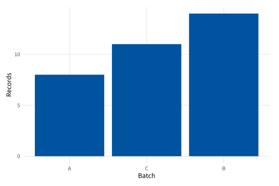
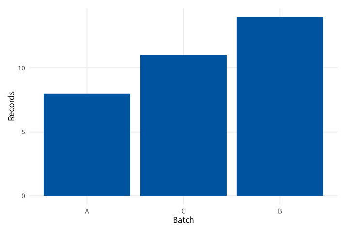
Copy link GGP-06-002 Rank categories by their totals Reorder uses the supplied totals to determine category order. Use it to show a count ranking while preserving the original names.
Back to diagram overview Compare with GGP-06-001 · Count the input rows .
Complete R / ggplot2 source source ( "config/style.R" )
d <- data.frame ( batch = c ( "A" , "B" , "C" ), n = c ( 8 , 14 , 11 ))
p <- ggplot ( d , aes ( reorder ( batch , n ), n )) + geom_col ( fill = "#00549F" ) +
labs ( x = "Batch" , y = "Records" )
export_plot ( p , "GGP-06-002" )
Parameter Meaning in this example reorder(batch,n)Arrange batch names by their supplied totals.
Render this diagram examples/GGP-06-002.R
Try changing: Use -n to reverse the ranking.
Actual output GGP-06-002 · R / ggplot2 native output R / ggplot2 · exit 0
Native compiler log Standard output Download: Source · Source + configuration ZIP · SVG · Native PDF · PNG
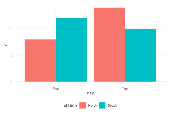
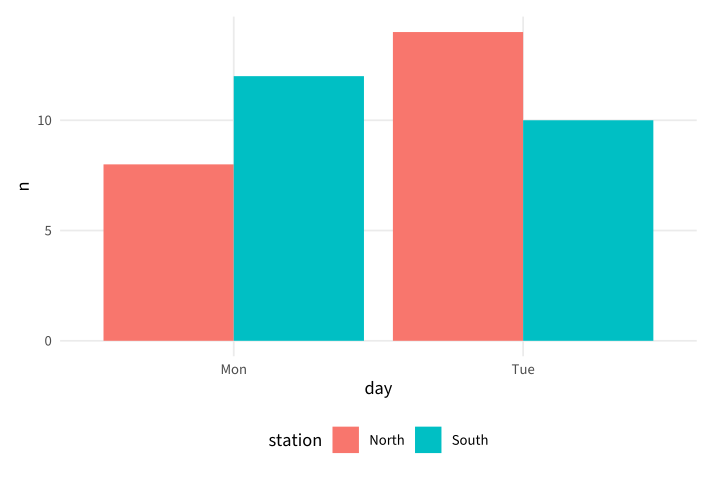
Copy link GGP-06-003 Place grouped bars side by side A dodge position separates groups within a category. Use it when the reader needs to compare station counts for the same day.
Back to diagram overview Compare with GGP-06-002 · Rank categories by their totals .
Complete R / ggplot2 source source ( "config/style.R" )
d <- data.frame ( day = rep ( c ( "Mon" , "Tue" ), each = 2 ),
station = rep ( c ( "North" , "South" ), 2 ), n = c ( 8 , 12 , 14 , 10 ))
p <- ggplot ( d , aes ( day , n , fill = station )) + geom_col ( position = "dodge" )
export_plot ( p , "GGP-06-003" )
Parameter Meaning in this example position="dodge"Place the two station bars beside each other.
Render this diagram examples/GGP-06-003.R
Try changing: Increase the South Tuesday count to 16.
Actual output GGP-06-003 · R / ggplot2 native output R / ggplot2 · exit 0
Native compiler log Standard output Download: Source · Source + configuration ZIP · SVG · Native PDF · PNG
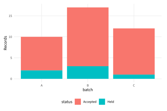
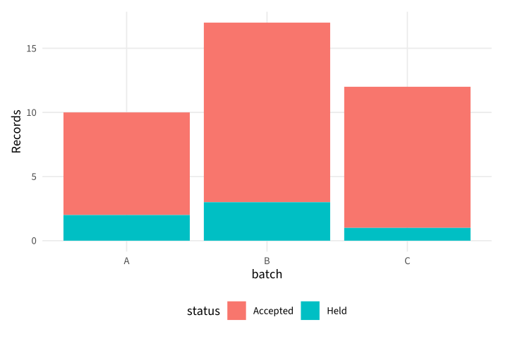
Copy link GGP-06-004 Stack parts of a total A stacked column keeps each component attached to its total. Use it when accepted and held records exhaust the supplied batch population.
Back to diagram overview Compare with GGP-06-003 · Place grouped bars side by side .
Complete R / ggplot2 source source ( "config/style.R" )
d <- data.frame ( batch = rep ( c ( "A" , "B" , "C" ), each = 2 ),
status = rep ( c ( "Accepted" , "Held" ), 3 ), n = c ( 8 , 2 , 14 , 3 , 11 , 1 ))
p <- ggplot ( d , aes ( batch , n , fill = status )) + geom_col () + labs ( y = "Records" )
export_plot ( p , "GGP-06-004" )
Parameter Meaning in this example fill=statusIdentify the two components of each stack.
Render this diagram examples/GGP-06-004.R
Try changing: Change batch B Held from 3 to 5.
Actual output GGP-06-004 · R / ggplot2 native output R / ggplot2 · exit 0
Native compiler log Standard output Download: Source · Source + configuration ZIP · SVG · Native PDF · PNG
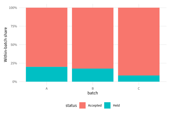
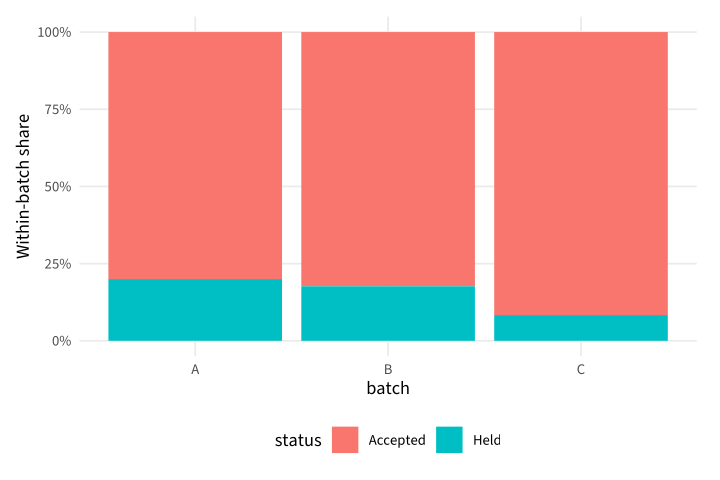
Copy link GGP-06-005 Normalize each batch to a whole A fill position divides by each stack's total. Use it when composition is the question, and retain the original counts in the complete source.
Back to diagram overview Compare with GGP-06-004 · Stack parts of a total .
Complete R / ggplot2 source source ( "config/style.R" )
d <- data.frame ( batch = rep ( c ( "A" , "B" , "C" ), each = 2 ),
status = rep ( c ( "Accepted" , "Held" ), 3 ), n = c ( 8 , 2 , 14 , 3 , 11 , 1 ))
p <- ggplot ( d , aes ( batch , n , fill = status )) + geom_col ( position = "fill" ) +
scale_y_continuous ( labels = function ( x ) paste0 ( 100 * x , "%" )) +
labs ( y = "Within-batch share" )
export_plot ( p , "GGP-06-005" )
Parameter Meaning in this example position="fill"Normalize every batch independently to a total height of one.
Render this diagram examples/GGP-06-005.R
Try changing: Increase a Held count and inspect the changed denominator.
Actual output GGP-06-005 · R / ggplot2 native output R / ggplot2 · exit 0
Native compiler log Standard output Download: Source · Source + configuration ZIP · SVG · Native PDF · PNG
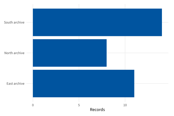
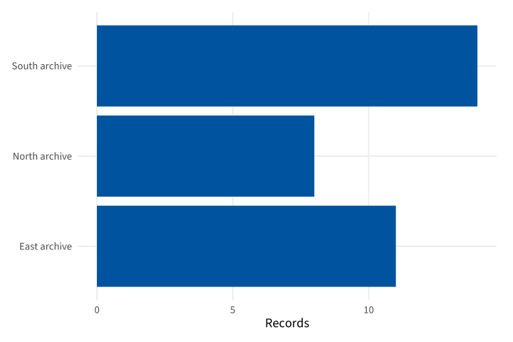
Copy link GGP-06-006 Put categories on the vertical axis A horizontal column chart leaves room for category names. Use an explicit value mapping instead of shortening meaningful station labels.
Back to diagram overview Compare with GGP-06-005 · Normalize each batch to a whole .
Complete R / ggplot2 source source ( "config/style.R" )
d <- data.frame ( station = c ( "North archive" , "South archive" , "East archive" ), n = c ( 8 , 14 , 11 ))
p <- ggplot ( d , aes ( n , station )) + geom_col ( fill = "#00549F" ) + labs ( x = "Records" , y = NULL )
export_plot ( p , "GGP-06-006" )
Parameter Meaning in this example aes(n,station)Place the numeric value horizontally and category vertically.
Render this diagram examples/GGP-06-006.R
Try changing: Order the stations by n.
Actual output GGP-06-006 · R / ggplot2 native output R / ggplot2 · exit 0
Native compiler log Standard output Download: Source · Source + configuration ZIP · SVG · Native PDF · PNG
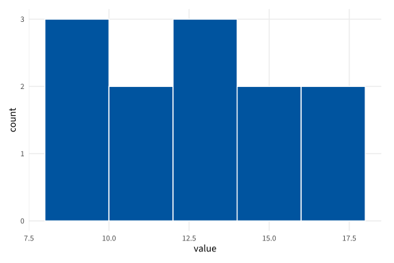
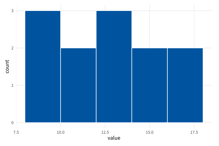
Copy link GGP-07-001 Fix histogram bins explicitly A histogram counts observations in intervals. Use a stated width, boundary and closure so the same values cannot silently move between bins.
Back to diagram overview Compare with GGP-06-001 · Count the input rows .
Complete R / ggplot2 source source ( "config/style.R" )
d <- data.frame ( value = c ( 8 , 9 , 9 , 10 , 11 , 12 , 12 , 13 , 14 , 15 , 16 , 18 ))
p <- ggplot ( d , aes ( value )) +
geom_histogram ( binwidth = 2 , boundary = 0 , closed = "left" ,
fill = "#00549F" , colour = "white" )
export_plot ( p , "GGP-07-001" )
Parameter Meaning in this example binwidth / boundary / closedUse two-unit intervals aligned to zero and closed on the left.
Render this diagram examples/GGP-07-001.R
Try changing: Change the bin width to 3.
Actual output GGP-07-001 · R / ggplot2 native output R / ggplot2 · exit 0
Native compiler log Standard output Download: Source · Source + configuration ZIP · SVG · Native PDF · PNG
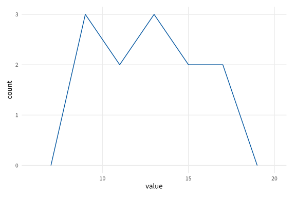
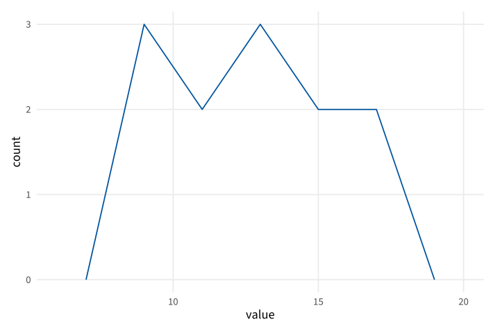
Copy link GGP-07-002 Draw counts as a frequency polygon A frequency polygon joins bin-center counts. Use the same bin definition as a histogram when comparing the two geometries.
Back to diagram overview Compare with GGP-07-001 · Fix histogram bins explicitly .
Complete R / ggplot2 source source ( "config/style.R" )
d <- data.frame ( value = c ( 8 , 9 , 9 , 10 , 11 , 12 , 12 , 13 , 14 , 15 , 16 , 18 ))
p <- ggplot ( d , aes ( value )) +
geom_freqpoly ( binwidth = 2 , boundary = 0 , closed = "left" , colour = "#00549F" )
export_plot ( p , "GGP-07-002" )
Parameter Meaning in this example geom_freqpoly()Join the supplied binning rule's center counts.
Render this diagram examples/GGP-07-002.R
Try changing: Change the width to 3 and compare the shape.
Actual output GGP-07-002 · R / ggplot2 native output R / ggplot2 · exit 0
Native compiler log Standard output Download: Source · Source + configuration ZIP · SVG · Native PDF · PNG
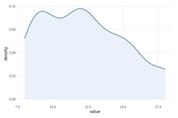
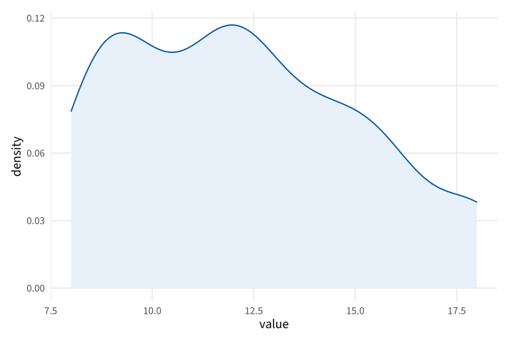
Copy link GGP-07-003 Fix a density bandwidth A density layer estimates a smooth distribution rather than counts. Use an explicit bandwidth so the smoothing choice is visible.
Back to diagram overview Compare with GGP-07-002 · Draw counts as a frequency polygon .
Complete R / ggplot2 source source ( "config/style.R" )
d <- data.frame ( value = c ( 8 , 9 , 9 , 10 , 11 , 12 , 12 , 13 , 14 , 15 , 16 , 18 ))
p <- ggplot ( d , aes ( value )) +
geom_density ( bw = 1 , fill = "#E8F1FA" , colour = "#00549F" )
export_plot ( p , "GGP-07-003" )
Parameter Meaning in this example bw=1Use a Gaussian smoothing bandwidth of one data unit.
Render this diagram examples/GGP-07-003.R
Try changing: Compare bandwidths .5 and 2.
Actual output GGP-07-003 · R / ggplot2 native output R / ggplot2 · exit 0
Native compiler log Standard output Download: Source · Source + configuration ZIP · SVG · Native PDF · PNG
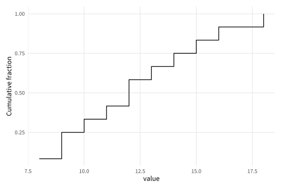
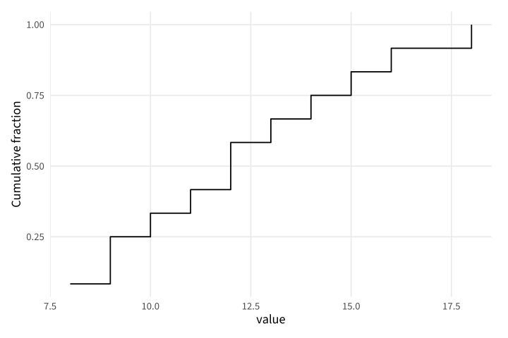
Copy link GGP-07-004 Show the cumulative distribution An empirical cumulative curve reports the fraction at or below each value. Use it to compare quantiles without selecting histogram bins.
Back to diagram overview Compare with GGP-07-003 · Fix a density bandwidth .
Complete R / ggplot2 source source ( "config/style.R" )
d <- data.frame ( value = c ( 8 , 9 , 9 , 10 , 11 , 12 , 12 , 13 , 14 , 15 , 16 , 18 ))
p <- ggplot ( d , aes ( value )) + stat_ecdf ( geom = "step" , pad = FALSE ) +
labs ( y = "Cumulative fraction" )
export_plot ( p , "GGP-07-004" )
Parameter Meaning in this example stat_ecdf()Compute the empirical cumulative distribution including ties.
Render this diagram examples/GGP-07-004.R
Try changing: Add another observation at value 12.
Actual output GGP-07-004 · R / ggplot2 native output R / ggplot2 · exit 0
Native compiler log Standard output Download: Source · Source + configuration ZIP · SVG · Native PDF · PNG
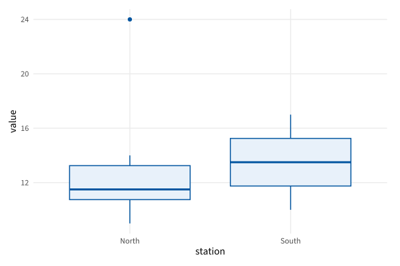
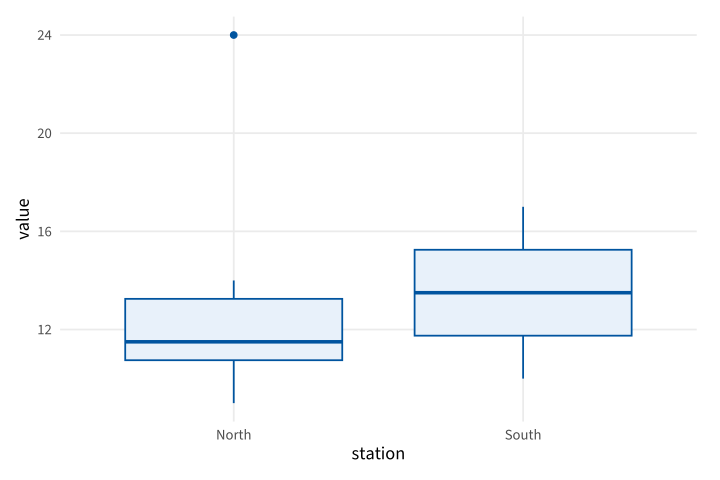
Copy link GGP-07-005 Expose the boxplot whisker rule A native boxplot estimates quartiles and flags distant observations. Here whiskers extend to observations within 1.5 interquartile ranges; they are not automatically the minimum and maximum.
Back to diagram overview Compare with GGP-07-004 · Show the cumulative distribution .
Complete R / ggplot2 source source ( "config/style.R" )
d <- data.frame ( station = rep ( c ( "North" , "South" ), each = 8 ),
value = c ( 9 , 10 , 11 , 11 , 12 , 13 , 14 , 24 , 10 , 11 , 12 , 13 , 14 , 15 , 16 , 17 ))
p <- ggplot ( d , aes ( station , value )) +
geom_boxplot ( coef = 1.5 , fill = "#E8F1FA" , colour = "#00549F" )
export_plot ( p , "GGP-07-005" )
Parameter Meaning in this example coef=1.5Set the interquartile-range multiplier for whisker limits.
Render this diagram examples/GGP-07-005.R
Try changing: Change coef to 2 and inspect the North outlier.
Actual output GGP-07-005 · R / ggplot2 native output R / ggplot2 · exit 0
Native compiler log Standard output Download: Source · Source + configuration ZIP · SVG · Native PDF · PNG
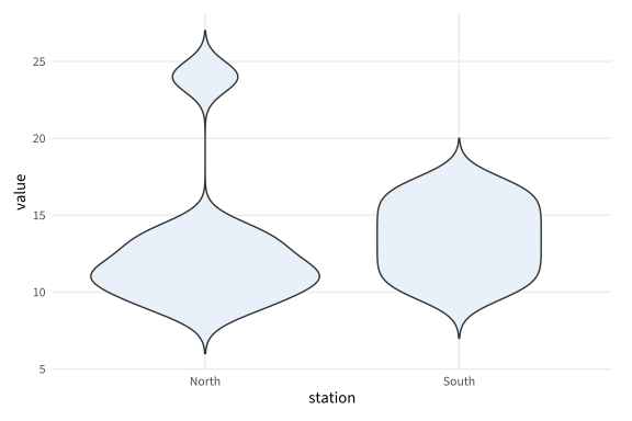
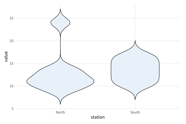
Copy link GGP-07-006 Compare native violin densities A violin mirrors a density estimate within each category. Use a common bandwidth and equal-area scaling when comparing station distributions.
Back to diagram overview Compare with GGP-07-005 · Expose the boxplot whisker rule .
Complete R / ggplot2 source source ( "config/style.R" )
d <- data.frame ( station = rep ( c ( "North" , "South" ), each = 8 ),
value = c ( 9 , 10 , 11 , 11 , 12 , 13 , 14 , 24 , 10 , 11 , 12 , 13 , 14 , 15 , 16 , 17 ))
p <- ggplot ( d , aes ( station , value )) +
geom_violin ( bw = 1 , trim = FALSE , scale = "area" , fill = "#E8F1FA" )
export_plot ( p , "GGP-07-006" )
Parameter Meaning in this example trim=FALSE / scale="area"Retain estimated tails and normalize the violin areas.
Render this diagram examples/GGP-07-006.R
Try changing: Change the bandwidth to 2.
Actual output GGP-07-006 · R / ggplot2 native output R / ggplot2 · exit 0
Native compiler log Standard output Download: Source · Source + configuration ZIP · SVG · Native PDF · PNG
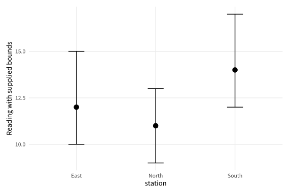
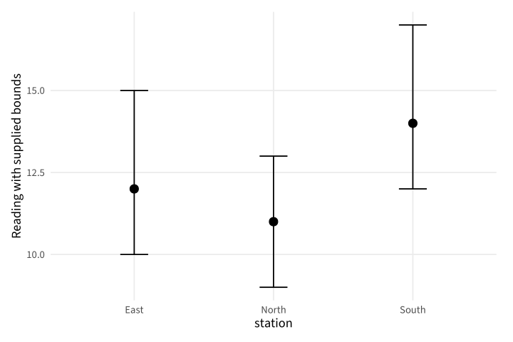
Copy link GGP-08-001 Draw supplied measurement bounds An error bar can display bounds provided with a reading. Use explicit lower and upper columns rather than implying an unstated confidence procedure.
Back to diagram overview Compare with GGP-03-005 · Show a supplied range as a band .
Complete R / ggplot2 source source ( "config/style.R" )
d <- data.frame ( station = c ( "North" , "South" , "East" ), mean = c ( 11 , 14 , 12 ),
low = c ( 9 , 12 , 10 ), high = c ( 13 , 17 , 15 ))
p <- ggplot ( d , aes ( station , mean )) + geom_point ( size = 3 ) +
geom_errorbar ( aes ( ymin = low , ymax = high ), width = . 2 ) +
labs ( y = "Reading with supplied bounds" )
export_plot ( p , "GGP-08-001" )
Parameter Meaning in this example ymin / ymaxRead the supplied interval columns directly.
Render this diagram examples/GGP-08-001.R
Try changing: Widen the East upper bound to 17.
Actual output GGP-08-001 · R / ggplot2 native output R / ggplot2 · exit 0
Native compiler log Standard output Download: Source · Source + configuration ZIP · SVG · Native PDF · PNG
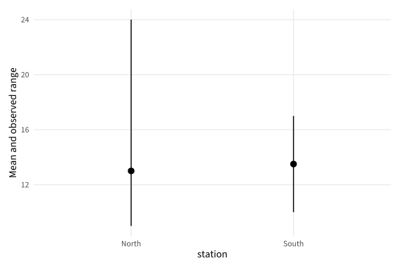
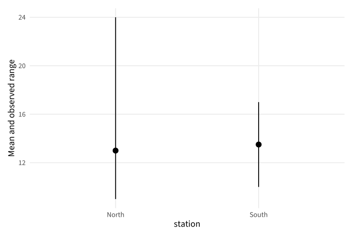
Copy link GGP-08-002 Summarize raw groups with a layer A summary layer can calculate a center from the supplied observations. Here the interval is the observed range, with no claim of statistical confidence.
Back to diagram overview Compare with GGP-08-001 · Draw supplied measurement bounds .
Complete R / ggplot2 source source ( "config/style.R" )
d <- data.frame ( station = rep ( c ( "North" , "South" ), each = 8 ),
value = c ( 9 , 10 , 11 , 11 , 12 , 13 , 14 , 24 , 10 , 11 , 12 , 13 , 14 , 15 , 16 , 17 ))
p <- ggplot ( d , aes ( station , value )) +
stat_summary ( fun = mean , fun.min = min , fun.max = max , geom = "pointrange" ) +
labs ( y = "Mean and observed range" )
export_plot ( p , "GGP-08-002" )
Parameter Meaning in this example fun / fun.min / fun.maxName the three explicit summary functions.
Render this diagram examples/GGP-08-002.R
Try changing: Replace mean with median.
Actual output GGP-08-002 · R / ggplot2 native output R / ggplot2 · exit 0
Native compiler log Standard output Download: Source · Source + configuration ZIP · SVG · Native PDF · PNG
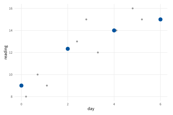
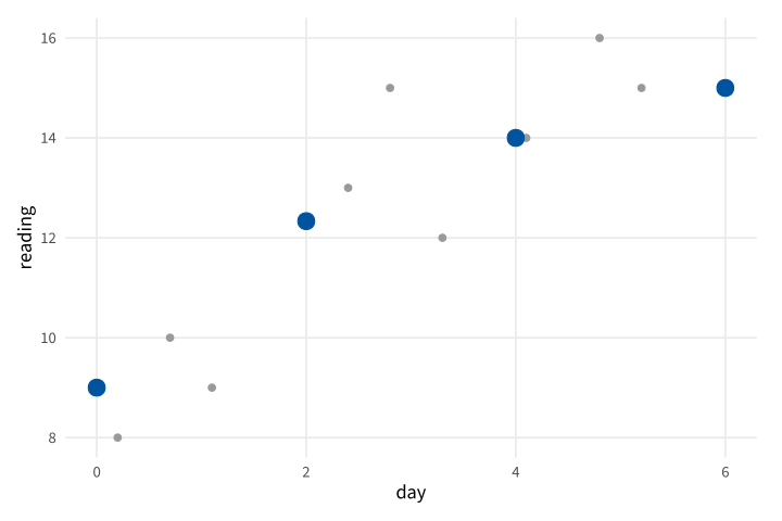
Copy link GGP-08-003 Summarize observations in fixed bins A binned summary groups a continuous coordinate into intervals. Use a stated bin width when irregularly spaced observations need a comparable local mean.
Back to diagram overview Compare with GGP-08-002 · Summarize raw groups with a layer .
Complete R / ggplot2 source source ( "config/style.R" )
d <- data.frame ( day = c ( . 2 , . 7 , 1.1 , 2.4 , 2.8 , 3.3 , 4.1 , 4.8 , 5.2 ),
reading = c ( 8 , 10 , 9 , 13 , 15 , 12 , 14 , 16 , 15 ))
p <- ggplot ( d , aes ( day , reading )) + geom_point ( colour = "grey60" ) +
stat_summary_bin ( fun = mean , geom = "point" , binwidth = 2 , colour = "#00549F" , size = 4 )
export_plot ( p , "GGP-08-003" )
Parameter Meaning in this example stat_summary_bin()Calculate the supplied function within each fixed-width bin.
Render this diagram examples/GGP-08-003.R
Try changing: Change binwidth to 1.
Actual output GGP-08-003 · R / ggplot2 native output R / ggplot2 · exit 0
Native compiler log Standard output Download: Source · Source + configuration ZIP · SVG · Native PDF · PNG
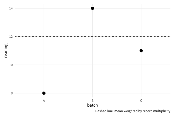
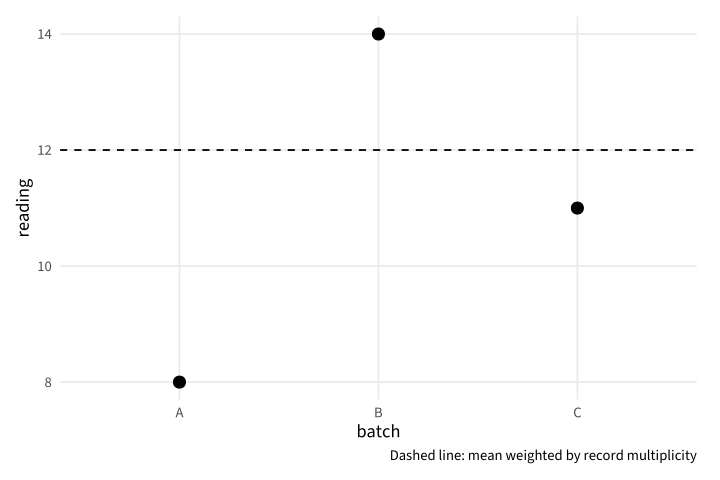
Copy link GGP-08-004 State a weighted mean explicitly Weights change the contribution of each supplied value. Use an explicit calculation and caption when weights represent known record multiplicities.
Back to diagram overview Compare with GGP-08-003 · Summarize observations in fixed bins .
Complete R / ggplot2 source source ( "config/style.R" )
d <- data.frame ( batch = c ( "A" , "B" , "C" ), reading = c ( 8 , 14 , 11 ), weight = c ( 1 , 3 , 2 ))
m <- weighted.mean ( d $ reading , d $ weight )
p <- ggplot ( d , aes ( batch , reading )) + geom_point ( size = 3 ) +
geom_hline ( yintercept = m , linetype = "dashed" ) +
labs ( caption = "Dashed line: mean weighted by record multiplicity" )
export_plot ( p , "GGP-08-004" )
Parameter Meaning in this example weighted.mean()Calculate the center using the supplied multiplicities.
Render this diagram examples/GGP-08-004.R
Try changing: Change batch B weight to 1.
Actual output GGP-08-004 · R / ggplot2 native output R / ggplot2 · exit 0
Native compiler log Standard output Download: Source · Source + configuration ZIP · SVG · Native PDF · PNG
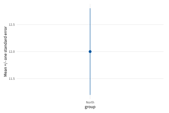
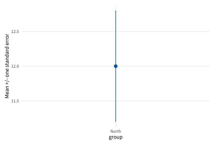
Copy link GGP-08-005 Calculate one standard error A standard error describes variability of the sample mean under the stated sampling interpretation. This example displays one standard error on each side of the mean, not a confidence interval.
Back to diagram overview Compare with GGP-08-004 · State a weighted mean explicitly .
Complete R / ggplot2 source source ( "config/style.R" )
values <- c ( 9 , 10 , 11 , 11 , 12 , 13 , 14 , 16 )
m <- mean ( values ); se <- sd ( values ) / sqrt ( length ( values ))
d <- data.frame ( group = "North" , mean = m , low = m - se , high = m + se )
p <- ggplot ( d , aes ( group , mean , ymin = low , ymax = high )) +
geom_pointrange ( colour = "#00549F" ) + labs ( y = "Mean +/- one standard error" )
export_plot ( p , "GGP-08-005" )
Parameter Meaning in this example sd(x)/sqrt(n)Calculate the standard error of the supplied sample mean.
Render this diagram examples/GGP-08-005.R
Try changing: Add another value of 16 and recalculate.
Actual output GGP-08-005 · R / ggplot2 native output R / ggplot2 · exit 0
Native compiler log Standard output Download: Source · Source + configuration ZIP · SVG · Native PDF · PNG
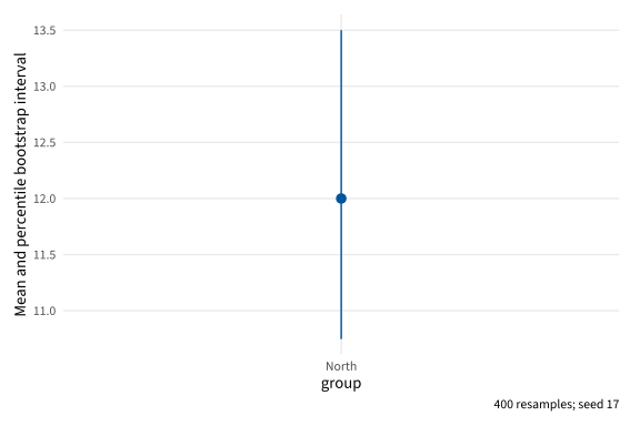
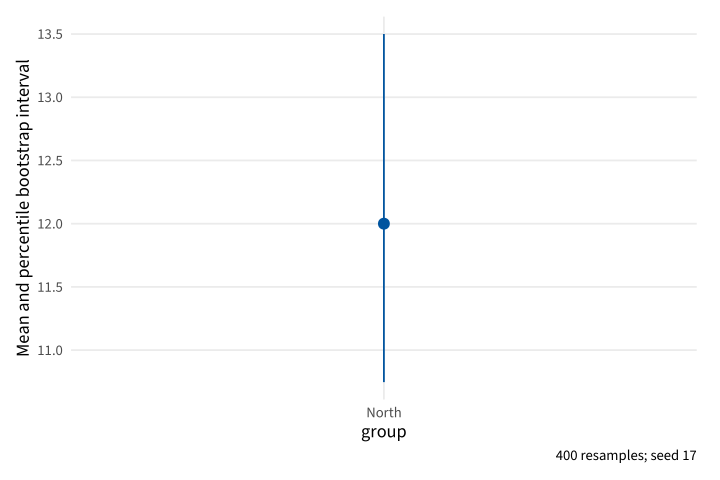
Copy link GGP-08-006 Make a reproducible bootstrap interval Resampling can provide an illustrative percentile interval for the mean. Use an explicit seed, number of resamples and quantile rule so the computational procedure can be reproduced.
Back to diagram overview Compare with GGP-08-005 · Calculate one standard error .
Complete R / ggplot2 source source ( "config/style.R" )
RNGkind ( "Mersenne-Twister" , "Inversion" , "Rejection" ); set.seed ( 17 )
values <- c ( 9 , 10 , 11 , 11 , 12 , 13 , 14 , 16 )
means <- replicate ( 400 , mean ( sample ( values , replace = TRUE )))
bounds <- quantile ( means , c ( . 025 , . 975 ), type = 7 )
d <- data.frame ( group = "North" , mean = mean ( values ), low = bounds [ 1 ], high = bounds [ 2 ])
p <- ggplot ( d , aes ( group , mean , ymin = low , ymax = high )) +
geom_pointrange ( colour = "#00549F" ) +
labs ( y = "Mean and percentile bootstrap interval" , caption = "400 resamples; seed 17" )
export_plot ( p , "GGP-08-006" )
Parameter Meaning in this example replicate / sampleGenerate the stated number of replacement samples. type=7Use an explicit interpolated quantile rule.
Render this diagram examples/GGP-08-006.R
Try changing: Increase the resample count to 800 and update the caption.
Actual output GGP-08-006 · R / ggplot2 native output R / ggplot2 · exit 0
Native compiler log Standard output Download: Source · Source + configuration ZIP · SVG · Native PDF · PNG
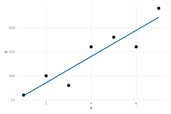
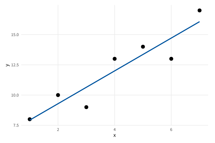
Copy link GGP-09-001 Fit a stated linear trend A smoothing layer can fit an explicit least-squares model. Keep the observations visible and state the model instead of implying that the line is another measured series.
Back to diagram overview Compare with GGP-03-001 · Show samples on their trend .
Complete R / ggplot2 source source ( "config/style.R" )
d <- data.frame ( x = 1 : 7 , y = c ( 8 , 10 , 9 , 13 , 14 , 13 , 17 ))
p <- ggplot ( d , aes ( x , y )) + geom_point ( size = 3 ) +
geom_smooth ( method = "lm" , formula = y ~ x , se = FALSE , colour = "#00549F" )
export_plot ( p , "GGP-09-001" )
Parameter Meaning in this example method="lm" / formula=y~xFit the stated linear mean model.
Render this diagram examples/GGP-09-001.R
Try changing: Change one observation and inspect the fitted line.
Actual output GGP-09-001 · R / ggplot2 native output R / ggplot2 · exit 0
Native compiler log Standard output Download: Source · Source + configuration ZIP · SVG · Native PDF · PNG
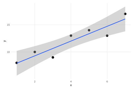
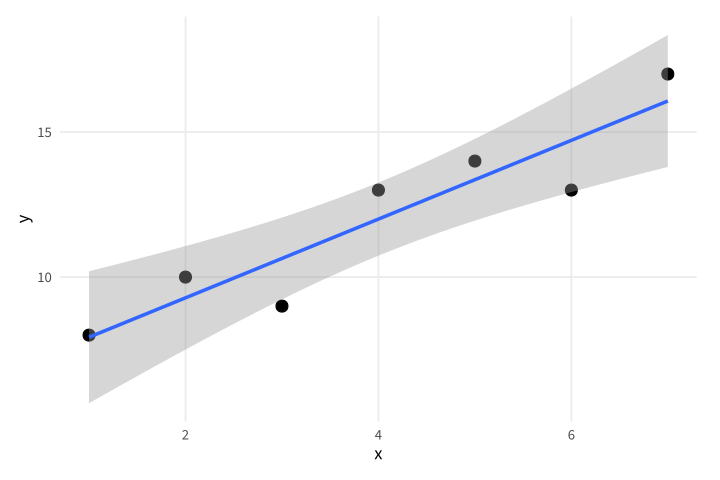
Copy link GGP-09-002 Show uncertainty in the fitted mean The smooth layer can draw a confidence band for the model mean. This is a model-based interval under linear-model assumptions, not a prediction interval for individual readings.
Back to diagram overview Compare with GGP-09-001 · Fit a stated linear trend .
Complete R / ggplot2 source source ( "config/style.R" )
d <- data.frame ( x = 1 : 7 , y = c ( 8 , 10 , 9 , 13 , 14 , 13 , 17 ))
p <- ggplot ( d , aes ( x , y )) + geom_point ( size = 3 ) +
geom_smooth ( method = "lm" , formula = y ~ x , se = TRUE , level = . 95 )
export_plot ( p , "GGP-09-002" )
Parameter Meaning in this example se / levelDisplay the stated confidence level for the fitted mean.
Render this diagram examples/GGP-09-002.R
Try changing: Change level to .8.
Actual output GGP-09-002 · R / ggplot2 native output R / ggplot2 · exit 0
Native compiler log Standard output Download: Source · Source + configuration ZIP · SVG · Native PDF · PNG
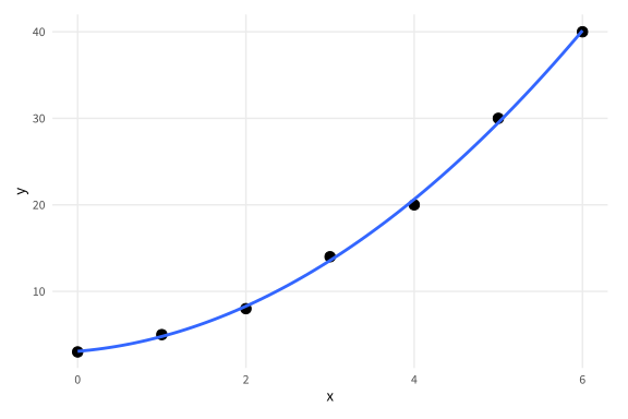
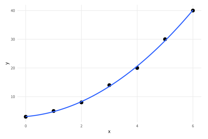
Copy link GGP-09-003 Fit a quadratic reference curve An explicit polynomial formula changes the model while leaving the observations intact. Use it for an illustrative curved relationship with enough data to inspect the fit.
Back to diagram overview Compare with GGP-09-002 · Show uncertainty in the fitted mean .
Complete R / ggplot2 source source ( "config/style.R" )
d <- data.frame ( x = 0 : 6 , y = c ( 3 , 5 , 8 , 14 , 20 , 30 , 40 ))
p <- ggplot ( d , aes ( x , y )) + geom_point ( size = 3 ) +
geom_smooth ( method = "lm" , formula = y ~ poly ( x , 2 , raw = TRUE ), se = FALSE )
export_plot ( p , "GGP-09-003" )
Parameter Meaning in this example poly(x,2,raw=TRUE)Fit an intercept, linear term and squared term.
Render this diagram examples/GGP-09-003.R
Try changing: Change the middle observation from 14 to 20.
Actual output GGP-09-003 · R / ggplot2 native output R / ggplot2 · exit 0
Native compiler log Standard output Download: Source · Source + configuration ZIP · SVG · Native PDF · PNG
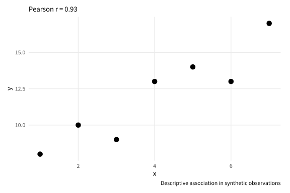
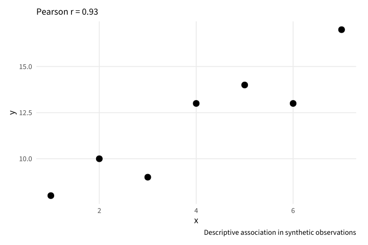
Copy link GGP-09-004 Report the correlation explicitly A computed correlation can accompany a scatterplot without replacing it. Use a caption that avoids interpreting this descriptive association as a causal effect.
Back to diagram overview Compare with GGP-09-003 · Fit a quadratic reference curve .
Complete R / ggplot2 source source ( "config/style.R" )
d <- data.frame ( x = 1 : 7 , y = c ( 8 , 10 , 9 , 13 , 14 , 13 , 17 ))
r <- cor ( d $ x , d $ y )
p <- ggplot ( d , aes ( x , y )) + geom_point ( size = 3 ) +
labs ( subtitle = sprintf ( "Pearson r = %.2f" , r ),
caption = "Descriptive association in synthetic observations" )
export_plot ( p , "GGP-09-004" )
Parameter Meaning in this example cor()Calculate the displayed Pearson correlation from the same rows.
Render this diagram examples/GGP-09-004.R
Try changing: Change the seventh y value to 8.
Actual output GGP-09-004 · R / ggplot2 native output R / ggplot2 · exit 0
Native compiler log Standard output Download: Source · Source + configuration ZIP · SVG · Native PDF · PNG
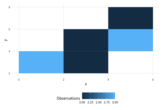
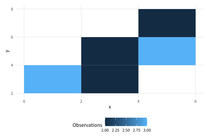
Copy link GGP-09-005 Count observations in two-dimensional bins A binned layer aggregates overlapping observations into cells. Use explicit bin widths and a count legend so color has a defined meaning.
Back to diagram overview Compare with GGP-09-004 · Report the correlation explicitly .
Complete R / ggplot2 source source ( "config/style.R" )
d <- data.frame ( x = c ( 1 , 1.2 , 1.5 , 2.4 , 2.7 , 3.1 , 3.2 , 4.2 , 4.5 , 5.1 , 5.4 , 5.6 ),
y = c ( 2 , 2.2 , 2.5 , 3.8 , 4.1 , 3.5 , 4.2 , 5.1 , 5.3 , 6.1 , 5.8 , 6.4 ))
p <- ggplot ( d , aes ( x , y )) + geom_bin_2d ( binwidth = c ( 2 , 2 )) +
labs ( fill = "Observations" )
export_plot ( p , "GGP-09-005" )
Parameter Meaning in this example binwidth=c(2,2)Count rows within the specified rectangular data cells.
Render this diagram examples/GGP-09-005.R
Try changing: Change both bin widths to one.
Actual output GGP-09-005 · R / ggplot2 native output R / ggplot2 · exit 0
Native compiler log Standard output Download: Source · Source + configuration ZIP · SVG · Native PDF · PNG
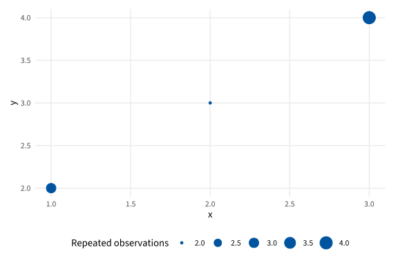
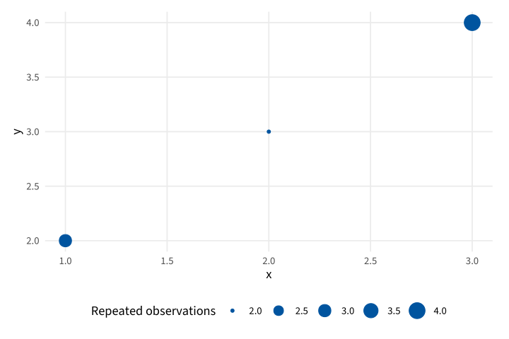
Copy link GGP-09-006 Expose coincident observations A count layer combines observations at identical coordinates. Use it when repeated discrete readings would otherwise hide under one point.
Back to diagram overview Compare with GGP-09-005 · Count observations in two-dimensional bins .
Complete R / ggplot2 source source ( "config/style.R" )
d <- data.frame ( x = c ( 1 , 1 , 1 , 2 , 2 , 3 , 3 , 3 , 3 ), y = c ( 2 , 2 , 2 , 3 , 3 , 4 , 4 , 4 , 4 ))
p <- ggplot ( d , aes ( x , y )) + geom_count ( colour = "#00549F" ) +
labs ( size = "Repeated observations" )
export_plot ( p , "GGP-09-006" )
Parameter Meaning in this example geom_count()Represent coordinate multiplicity with point area.
Render this diagram examples/GGP-09-006.R
Try changing: Add another row at 2,3.
Actual output GGP-09-006 · R / ggplot2 native output R / ggplot2 · exit 0
Native compiler log Standard output Download: Source · Source + configuration ZIP · SVG · Native PDF · PNG
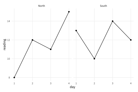
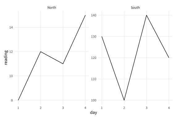
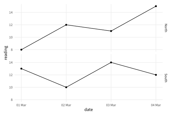
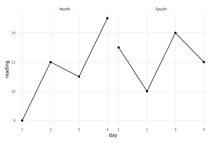
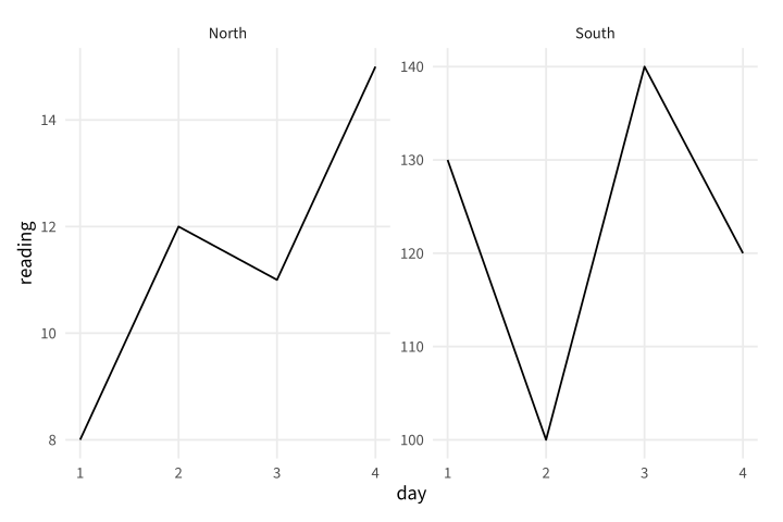
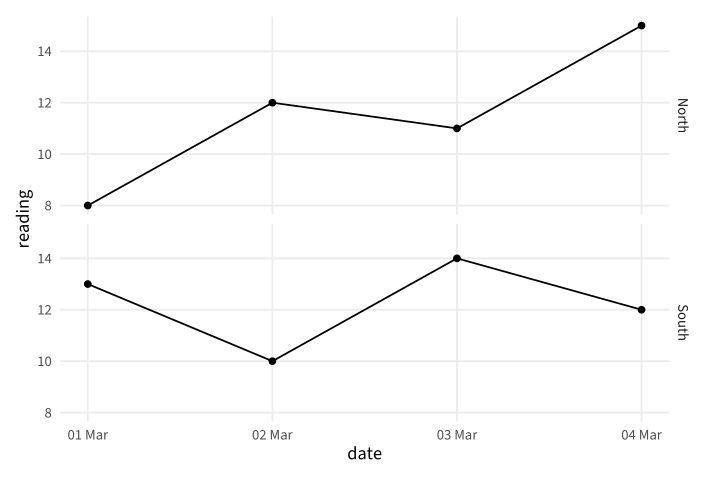
Copy link GGP-10-001 Give each station its own panel A wrapped facet splits a long table by station. Use common scales when the heights should remain directly comparable.
Back to diagram overview Compare with GGP-02-002 · Keep series in a long table .
Complete R / ggplot2 source source ( "config/style.R" )
d <- data.frame ( station = rep ( c ( "North" , "South" ), each = 4 ),
day = rep ( 1 : 4 , 2 ), reading = c ( 8 , 12 , 11 , 15 , 13 , 10 , 14 , 12 ))
p <- ggplot ( d , aes ( day , reading )) + geom_line () + geom_point () +
facet_wrap ( vars ( station ))
export_plot ( p , "GGP-10-001" )
Parameter Meaning in this example facet_wrap()Arrange one panel for each station.
Render this diagram examples/GGP-10-001.R
Try changing: Change the wrap to one column.
Actual output GGP-10-001 · R / ggplot2 native output R / ggplot2 · exit 0
Native compiler log Standard output Download: Source · Source + configuration ZIP · SVG · Native PDF · PNG
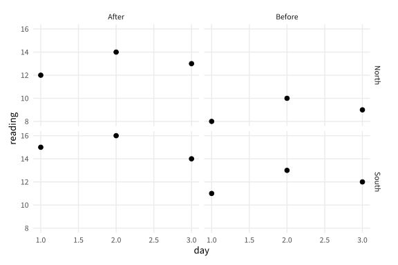
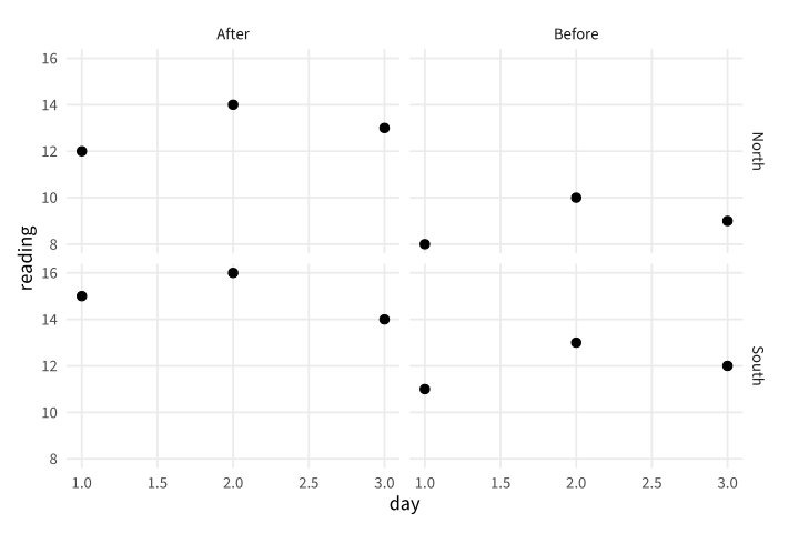
Copy link GGP-10-002 Facet by two grouping variables A facet grid assigns one variable to rows and another to columns. Use it to make both station and measurement phase visible.
Back to diagram overview Compare with GGP-10-001 · Give each station its own panel .
Complete R / ggplot2 source source ( "config/style.R" )
d <- data.frame ( station = rep ( c ( "North" , "South" ), each = 6 ),
phase = rep ( rep ( c ( "Before" , "After" ), each = 3 ), 2 ),
day = rep ( 1 : 3 , 4 ), reading = c ( 8 , 10 , 9 , 12 , 14 , 13 , 11 , 13 , 12 , 15 , 16 , 14 ))
p <- ggplot ( d , aes ( day , reading )) + geom_point ( size = 2 ) +
facet_grid ( station ~ phase )
export_plot ( p , "GGP-10-002" )
Parameter Meaning in this example facet_grid(station~phase)Cross station rows with phase columns.
Render this diagram examples/GGP-10-002.R
Try changing: Exchange the row and column variables.
Actual output GGP-10-002 · R / ggplot2 native output R / ggplot2 · exit 0
Native compiler log Standard output Download: Source · Source + configuration ZIP · SVG · Native PDF · PNG
Copy link GGP-10-003 Allow separate value scales Free vertical scales emphasize within-panel variation. State this choice because equal heights in the two panels no longer mean equal values.
Back to diagram overview Compare with GGP-10-002 · Facet by two grouping variables .
Complete R / ggplot2 source source ( "config/style.R" )
d <- data.frame ( station = rep ( c ( "North" , "South" ), each = 4 ),
day = rep ( 1 : 4 , 2 ), reading = c ( 8 , 12 , 11 , 15 , 13 , 10 , 14 , 12 ))
d $ reading [ d $ station == "South" ] <- 10 * d $ reading [ d $ station == "South" ]
p <- ggplot ( d , aes ( day , reading )) + geom_line () +
facet_wrap ( vars ( station ), scales = "free_y" )
export_plot ( p , "GGP-10-003" )
Parameter Meaning in this example scales="free_y"Fit a separate vertical range in each panel.
Render this diagram examples/GGP-10-003.R
Try changing: Return scales to fixed.
Actual output GGP-10-003 · R / ggplot2 native output R / ggplot2 · exit 0
Native compiler log Standard output Download: Source · Source + configuration ZIP · SVG · Native PDF · PNG
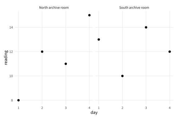
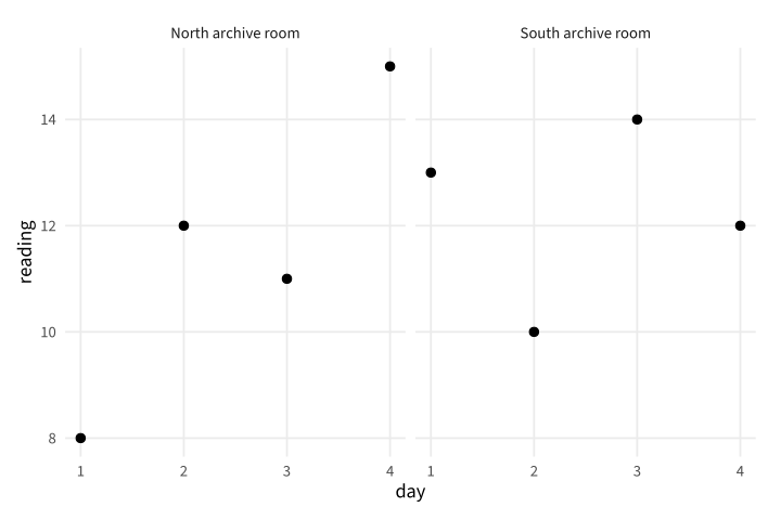
Copy link GGP-10-004 Write readable panel labels A labeller can expand stored group codes for readers. Use it to preserve concise data identifiers while explaining the station in the figure.
Back to diagram overview Compare with GGP-10-003 · Allow separate value scales .
Complete R / ggplot2 source source ( "config/style.R" )
d <- data.frame ( station = rep ( c ( "North" , "South" ), each = 4 ),
day = rep ( 1 : 4 , 2 ), reading = c ( 8 , 12 , 11 , 15 , 13 , 10 , 14 , 12 ))
p <- ggplot ( d , aes ( day , reading )) + geom_point ( size = 2 ) +
facet_wrap ( vars ( station ), labeller = labeller ( station = c (
North = "North archive room" , South = "South archive room" )))
export_plot ( p , "GGP-10-004" )
Parameter Meaning in this example labeller()Map stored station values to readable strip labels.
Render this diagram examples/GGP-10-004.R
Try changing: Change the two display labels.
Actual output GGP-10-004 · R / ggplot2 native output R / ggplot2 · exit 0
Native compiler log Standard output Download: Source · Source + configuration ZIP · SVG · Native PDF · PNG
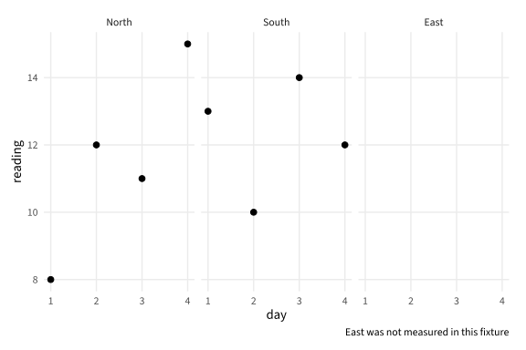
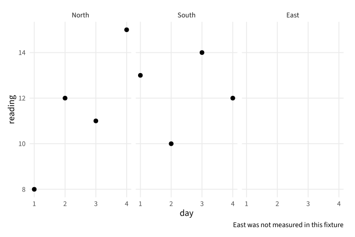
Copy link GGP-10-005 Retain an unmeasured category An unused factor level can remain as an explicitly empty panel. Use it to show that a planned station has no observations, rather than implying that its reading was zero.
Back to diagram overview Compare with GGP-10-004 · Write readable panel labels .
Complete R / ggplot2 source source ( "config/style.R" )
d <- data.frame ( station = rep ( c ( "North" , "South" ), each = 4 ),
day = rep ( 1 : 4 , 2 ), reading = c ( 8 , 12 , 11 , 15 , 13 , 10 , 14 , 12 ))
d $ station <- factor ( d $ station , levels = c ( "North" , "South" , "East" ))
p <- ggplot ( d , aes ( day , reading )) + geom_point ( size = 2 ) +
facet_wrap ( vars ( station ), drop = FALSE ) +
labs ( caption = "East was not measured in this fixture" )
export_plot ( p , "GGP-10-005" )
Parameter Meaning in this example drop=FALSERetain the declared category with no observed rows.
Render this diagram examples/GGP-10-005.R
Try changing: Set drop to TRUE and compare the inventory.
Actual output GGP-10-005 · R / ggplot2 native output R / ggplot2 · exit 0
Native compiler log Standard output Download: Source · Source + configuration ZIP · SVG · Native PDF · PNG
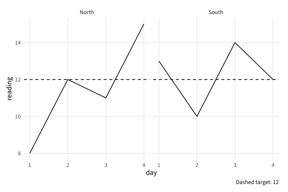
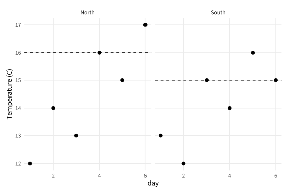
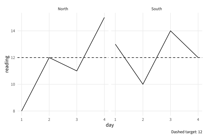
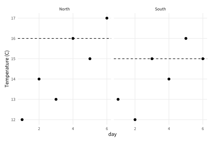
Copy link GGP-10-006 Repeat one reference across panels A layer with a fixed reference can appear in every facet. Use it when all stations share the same operational target.
Back to diagram overview Compare with GGP-10-005 · Retain an unmeasured category .
Complete R / ggplot2 source source ( "config/style.R" )
d <- data.frame ( station = rep ( c ( "North" , "South" ), each = 4 ),
day = rep ( 1 : 4 , 2 ), reading = c ( 8 , 12 , 11 , 15 , 13 , 10 , 14 , 12 ))
p <- ggplot ( d , aes ( day , reading )) + geom_line () +
geom_hline ( yintercept = 12 , linetype = "dashed" ) +
facet_wrap ( vars ( station )) + labs ( caption = "Dashed target: 12" )
export_plot ( p , "GGP-10-006" )
Parameter Meaning in this example Fixed reference layerRepeat the stated target in each station panel.
Render this diagram examples/GGP-10-006.R
Try changing: Change the target to 14 and update the caption.
Actual output GGP-10-006 · R / ggplot2 native output R / ggplot2 · exit 0
Native compiler log Standard output Download: Source · Source + configuration ZIP · SVG · Native PDF · PNG
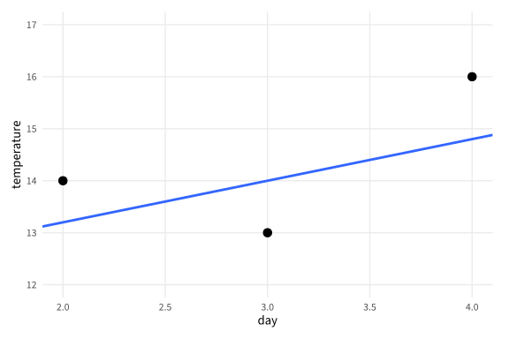
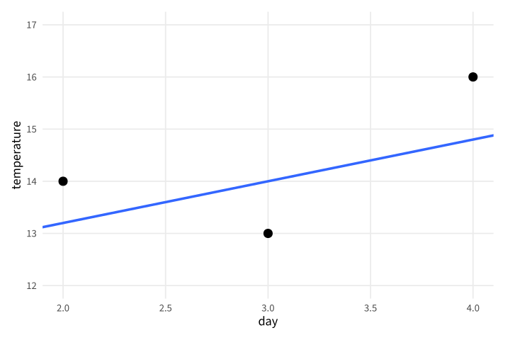
Copy link GGP-11-001 Zoom without discarding fit inputs A coordinate window changes what is visible after the model is fitted. Use it when the chart needs a closer view but the analysis should still use every supplied observation.
Back to diagram overview Compare with GGP-04-001 · Choose readable axis breaks .
Complete R / ggplot2 source source ( "config/style.R" )
d <- data.frame ( day = 1 : 5 , temperature = c ( 12 , 14 , 13 , 16 , 15 ))
p <- ggplot ( d , aes ( day , temperature )) + geom_point ( size = 3 ) +
geom_smooth ( method = "lm" , formula = y ~ x , se = FALSE ) +
coord_cartesian ( xlim = c ( 2 , 4 ), ylim = c ( 12 , 17 ))
export_plot ( p , "GGP-11-001" )
Parameter Meaning in this example coord_cartesian()Zoom after the layers and model have been calculated.
Render this diagram examples/GGP-11-001.R
Try changing: Widen the horizontal window to 1 through 5.
Actual output GGP-11-001 · R / ggplot2 native output R / ggplot2 · exit 0
Native compiler log Standard output Download: Source · Source + configuration ZIP · SVG · Native PDF · PNG
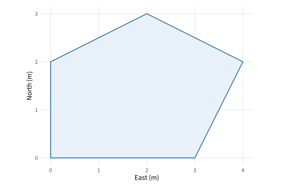
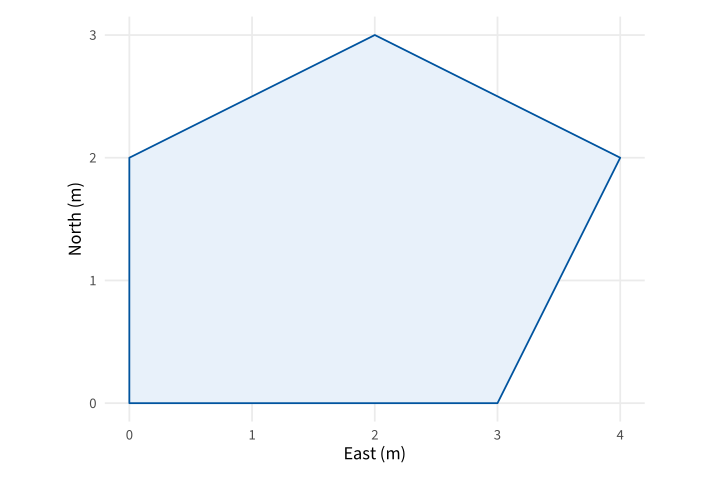
Copy link GGP-11-002 Preserve equal spatial units A fixed coordinate ratio makes one unit equally long on both axes. Use it for a field layout where geometric shape has a physical meaning.
Back to diagram overview Compare with GGP-11-001 · Zoom without discarding fit inputs .
Complete R / ggplot2 source source ( "config/style.R" )
d <- data.frame ( x = c ( 0 , 3 , 4 , 2 , 0 ), y = c ( 0 , 0 , 2 , 3 , 2 ))
p <- ggplot ( d , aes ( x , y )) + geom_polygon ( fill = "#E8F1FA" , colour = "#00549F" ) +
coord_fixed ( ratio = 1 ) + labs ( x = "East (m)" , y = "North (m)" )
export_plot ( p , "GGP-11-002" )
Parameter Meaning in this example ratio=1Use equal physical lengths for one horizontal and vertical data unit.
Render this diagram examples/GGP-11-002.R
Try changing: Change the ratio to .5 and inspect the distortion.
Actual output GGP-11-002 · R / ggplot2 native output R / ggplot2 · exit 0
Native compiler log Standard output Download: Source · Source + configuration ZIP · SVG · Native PDF · PNG
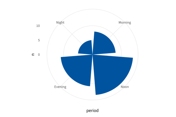
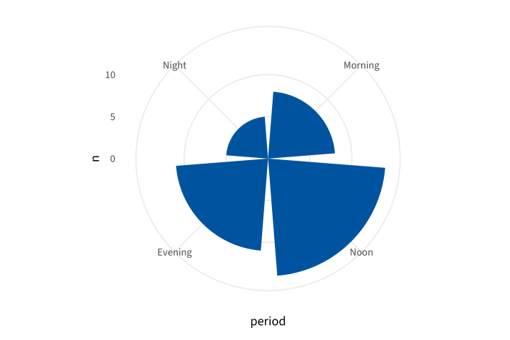
Copy link GGP-11-003 Lay out categories around a circle Polar coordinates transform the completed rectangular layers. Use them for a cyclic display only when readers can still interpret the category order and radial values.
Back to diagram overview Compare with GGP-11-002 · Preserve equal spatial units .
Complete R / ggplot2 source source ( "config/style.R" )
d <- data.frame ( period = factor ( c ( "Morning" , "Noon" , "Evening" , "Night" ),
levels = c ( "Morning" , "Noon" , "Evening" , "Night" )), n = c ( 8 , 14 , 11 , 5 ))
p <- ggplot ( d , aes ( period , n )) + geom_col ( fill = "#00549F" ) + coord_polar ()
export_plot ( p , "GGP-11-003" )
Parameter Meaning in this example coord_polar()Place category positions around the circle and counts radially.
Render this diagram examples/GGP-11-003.R
Try changing: Change the Night count to 9.
Actual output GGP-11-003 · R / ggplot2 native output R / ggplot2 · exit 0
Native compiler log Standard output Download: Source · Source + configuration ZIP · SVG · Native PDF · PNG
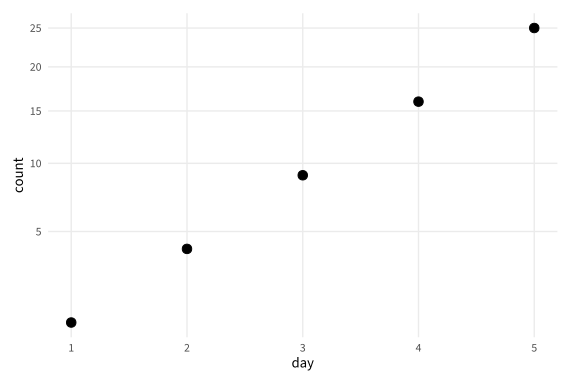
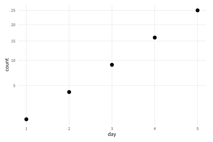
Copy link GGP-11-004 Transform coordinates after calculation A coordinate transformation changes the drawn scale after layer calculations. Use an explicit transform when that order differs from transforming the input data.
Back to diagram overview Compare with GGP-11-003 · Lay out categories around a circle .
Complete R / ggplot2 source source ( "config/style.R" )
d <- data.frame ( day = 1 : 5 , count = c ( 1 , 4 , 9 , 16 , 25 ))
p <- ggplot ( d , aes ( day , count )) + geom_point ( size = 3 ) +
coord_transform ( y = "sqrt" )
export_plot ( p , "GGP-11-004" )
Parameter Meaning in this example coord_transform(y="sqrt")Apply the square-root coordinate transformation to the completed layer.
Render this diagram examples/GGP-11-004.R
Try changing: Change the transform to log10, keeping all counts positive.
Actual output GGP-11-004 · R / ggplot2 native output R / ggplot2 · exit 0
Native compiler log Standard output Download: Source · Source + configuration ZIP · SVG · Native PDF · PNG
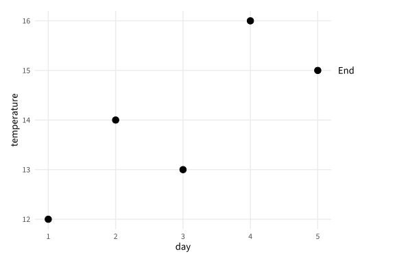
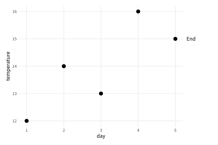
Copy link GGP-11-005 Put a note outside the panel Turning clipping off allows an annotation beyond a fixed viewing window. Add a margin so the exported page still contains the complete note.
Back to diagram overview Compare with GGP-11-004 · Transform coordinates after calculation .
Complete R / ggplot2 source source ( "config/style.R" )
d <- data.frame ( day = 1 : 5 , temperature = c ( 12 , 14 , 13 , 16 , 15 ))
p <- ggplot ( d , aes ( day , temperature )) + geom_point ( size = 3 ) +
annotate ( "text" , x = 5.3 , y = 15 , label = "End" , hjust = 0 ) +
coord_cartesian ( xlim = c ( 1 , 5 ), clip = "off" ) +
theme ( plot.margin = margin ( 12 , 70 , 12 , 12 ))
export_plot ( p , "GGP-11-005" )
Parameter Meaning in this example clip="off"Allow the annotation outside the panel window. plot.marginReserve real page space for the external note.
Render this diagram examples/GGP-11-005.R
Try changing: Change End to Final and inspect the page edge.
Actual output GGP-11-005 · R / ggplot2 native output R / ggplot2 · exit 0
Native compiler log Standard output Download: Source · Source + configuration ZIP · SVG · Native PDF · PNG
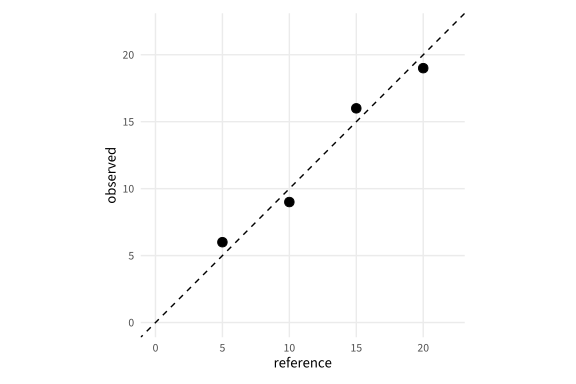
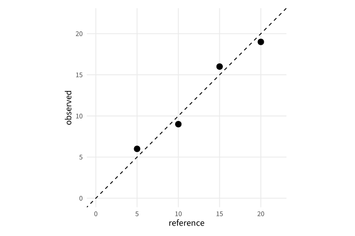
Copy link GGP-11-006 Compare calibration with an identity line An identity line marks equal supplied and measured values. Use equal axes so distance from that reference is not distorted by different physical scales.
Back to diagram overview Compare with GGP-11-005 · Put a note outside the panel .
Complete R / ggplot2 source source ( "config/style.R" )
d <- data.frame ( reference = c ( 5 , 10 , 15 , 20 ), observed = c ( 6 , 9 , 16 , 19 ))
p <- ggplot ( d , aes ( reference , observed )) + geom_point ( size = 3 ) +
geom_abline ( slope = 1 , intercept = 0 , linetype = "dashed" ) +
coord_equal ( xlim = c ( 0 , 22 ), ylim = c ( 0 , 22 ))
export_plot ( p , "GGP-11-006" )
Parameter Meaning in this example slope=1 / intercept=0Draw the equality reference, not a fitted regression.
Render this diagram examples/GGP-11-006.R
Try changing: Change one observed value to match its reference.
Actual output GGP-11-006 · R / ggplot2 native output R / ggplot2 · exit 0
Native compiler log Standard output Download: Source · Source + configuration ZIP · SVG · Native PDF · PNG
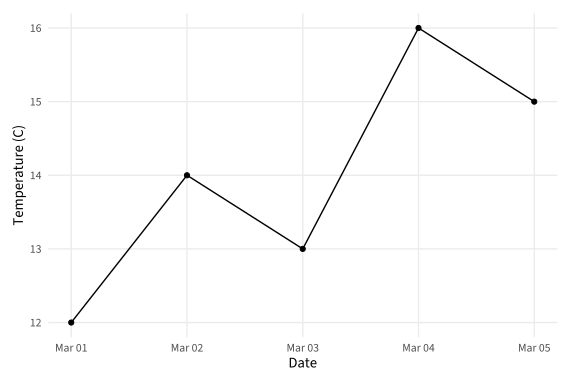
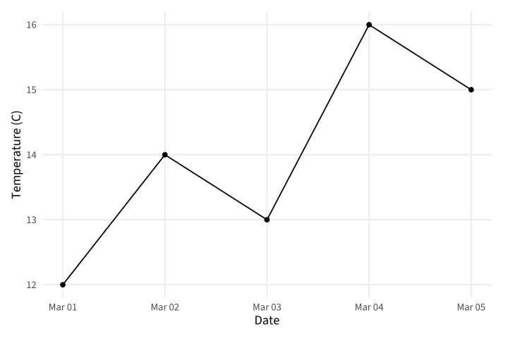
Copy link GGP-12-001 Use a calendar date axis A Date column provides calendar positions with native date labels. Use it when elapsed days must retain their actual dates.
Back to diagram overview Compare with GGP-01-004 · Connect an ordered series .
Complete R / ggplot2 source source ( "config/style.R" )
d <- data.frame ( day = as.Date ( "2025-03-01" ) +0 : 4 , temperature = c ( 12 , 14 , 13 , 16 , 15 ))
p <- ggplot ( d , aes ( day , temperature )) + geom_line () + geom_point () +
labs ( x = "Date" , y = "Temperature (C)" )
export_plot ( p , "GGP-12-001" )
Parameter Meaning in this example as.Date()Create fixed calendar dates rather than numeric category codes.
Render this diagram examples/GGP-12-001.R
Try changing: Move the starting date to April 1.
Actual output GGP-12-001 · R / ggplot2 native output R / ggplot2 · exit 0
Native compiler log Standard output Download: Source · Source + configuration ZIP · SVG · Native PDF · PNG
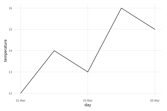
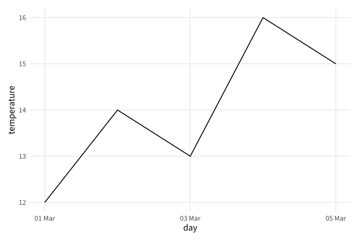
Copy link GGP-12-002 Choose date tick intervals A date scale can set both interval and displayed format. Use a fixed interval to keep labels legible across a short observation period.
Back to diagram overview Compare with GGP-12-001 · Use a calendar date axis .
Complete R / ggplot2 source source ( "config/style.R" )
d <- data.frame ( day = as.Date ( "2025-03-01" ) +0 : 4 , temperature = c ( 12 , 14 , 13 , 16 , 15 ))
p <- ggplot ( d , aes ( day , temperature )) + geom_line () +
scale_x_date ( date_breaks = "2 days" , date_labels = "%d %b" )
export_plot ( p , "GGP-12-002" )
Parameter Meaning in this example date_breaks / date_labelsSet the calendar interval and readable date format.
Render this diagram examples/GGP-12-002.R
Try changing: Change the tick interval to one day.
Actual output GGP-12-002 · R / ggplot2 native output R / ggplot2 · exit 0
Native compiler log Standard output Download: Source · Source + configuration ZIP · SVG · Native PDF · PNG
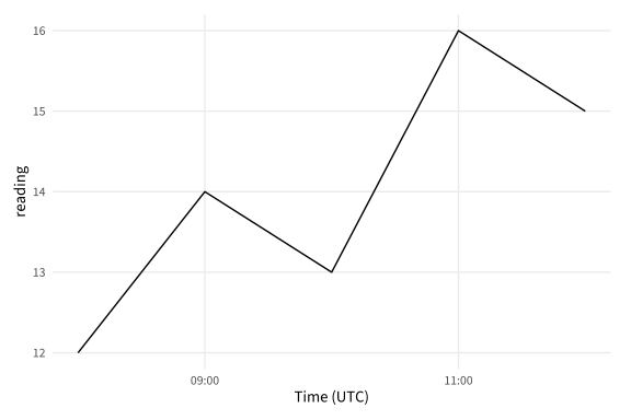
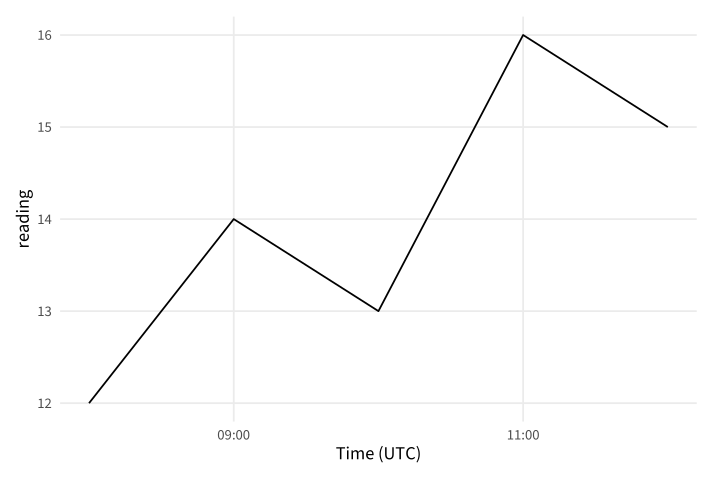
Copy link GGP-12-003 Pin timestamps to UTC A timestamp includes a time zone as well as a date. Use an explicit zone for construction and display so the same source does not shift between machines.
Back to diagram overview Compare with GGP-12-002 · Choose date tick intervals .
Complete R / ggplot2 source source ( "config/style.R" )
d <- data.frame ( time = as.POSIXct ( "2025-03-01 08:00" , tz = "UTC" ) + ( 0 : 4 ) * 3600 ,
reading = c ( 12 , 14 , 13 , 16 , 15 ))
p <- ggplot ( d , aes ( time , reading )) + geom_line () +
scale_x_datetime ( date_breaks = "2 hours" , date_labels = "%H:%M" , timezone = "UTC" ) +
labs ( x = "Time (UTC)" )
export_plot ( p , "GGP-12-003" )
Parameter Meaning in this example tz / timezoneUse UTC for both stored timestamps and tick labels.
Render this diagram examples/GGP-12-003.R
Try changing: Change the starting time to 06:00.
Actual output GGP-12-003 · R / ggplot2 native output R / ggplot2 · exit 0
Native compiler log Standard output Download: Source · Source + configuration ZIP · SVG · Native PDF · PNG
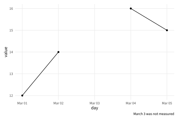
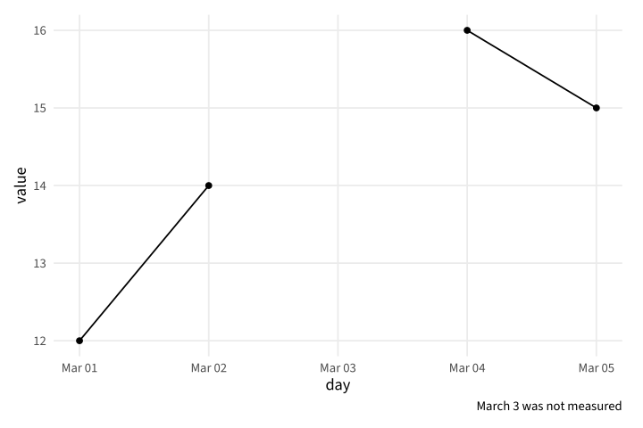
Copy link GGP-12-004 Complete a timeline before plotting An absent row is different from an explicit missing value. Merge the observations onto a complete daily calendar so the line exposes the unmeasured day.
Back to diagram overview Compare with GGP-12-003 · Pin timestamps to UTC .
Complete R / ggplot2 source source ( "config/style.R" )
observed <- data.frame ( day = as.Date ( "2025-03-01" ) + c ( 0 , 1 , 3 , 4 ), value = c ( 12 , 14 , 16 , 15 ))
calendar <- data.frame ( day = seq ( min ( observed $ day ), max ( observed $ day ), by = "day" ))
d <- merge ( calendar , observed , by = "day" , all.x = TRUE )
p <- ggplot ( d , aes ( day , value )) + geom_line ( na.rm = TRUE ) +
geom_point ( na.rm = TRUE ) + labs ( caption = "March 3 was not measured" )
export_plot ( p , "GGP-12-004" )
Parameter Meaning in this example all.x=TRUERetain every calendar date even when its value is missing.
Render this diagram examples/GGP-12-004.R
Try changing: Add an observation for March 3.
Actual output GGP-12-004 · R / ggplot2 native output R / ggplot2 · exit 0
Native compiler log Standard output Download: Source · Source + configuration ZIP · SVG · Native PDF · PNG
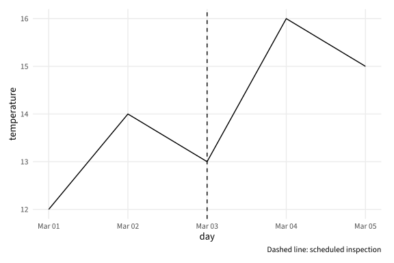
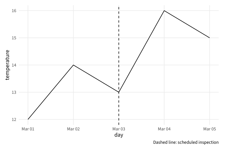
Copy link GGP-12-005 Mark a dated event A vertical reference can identify a known event on the calendar axis. Use a caption to name the event instead of implying it explains all nearby changes.
Back to diagram overview Compare with GGP-12-004 · Complete a timeline before plotting .
Complete R / ggplot2 source source ( "config/style.R" )
d <- data.frame ( day = as.Date ( "2025-03-01" ) +0 : 4 , temperature = c ( 12 , 14 , 13 , 16 , 15 ))
p <- ggplot ( d , aes ( day , temperature )) + geom_line () +
geom_vline ( xintercept = as.Date ( "2025-03-03" ), linetype = "dashed" ) +
labs ( caption = "Dashed line: scheduled inspection" )
export_plot ( p , "GGP-12-005" )
Parameter Meaning in this example Date-valued xinterceptPlace the event on the same calendar scale as the observations.
Render this diagram examples/GGP-12-005.R
Try changing: Move the inspection to March 4.
Actual output GGP-12-005 · R / ggplot2 native output R / ggplot2 · exit 0
Native compiler log Standard output Download: Source · Source + configuration ZIP · SVG · Native PDF · PNG
Copy link GGP-12-006 Align station calendars Facets can share a real date axis across groups. Use fixed date scales when the timing of observations should be compared directly.
Back to diagram overview Compare with GGP-12-005 · Mark a dated event .
Complete R / ggplot2 source source ( "config/style.R" )
d <- data.frame ( station = rep ( c ( "North" , "South" ), each = 4 ),
day = rep ( 1 : 4 , 2 ), reading = c ( 8 , 12 , 11 , 15 , 13 , 10 , 14 , 12 ))
d $ date <- as.Date ( "2025-03-01" ) + d $ day -1
p <- ggplot ( d , aes ( date , reading )) + geom_line () + geom_point () +
facet_grid ( station ~ . ) + scale_x_date ( date_labels = "%d %b" )
export_plot ( p , "GGP-12-006" )
Parameter Meaning in this example Shared date facetsCompare station timelines using the same calendar mapping.
Render this diagram examples/GGP-12-006.R
Try changing: Move the South dates forward by one day.
Actual output GGP-12-006 · R / ggplot2 native output R / ggplot2 · exit 0
Native compiler log Standard output Download: Source · Source + configuration ZIP · SVG · Native PDF · PNG
Copy link GGP-13-001 Draw a measured cell grid A tile layer gives each supplied cell a boundary. Use explicit coordinates when the grid represents field positions rather than an unordered table.
Back to diagram overview Compare with GGP-04-006 · Map a measured value continuously .
Complete R / ggplot2 source source ( "config/style.R" )
d <- expand.grid ( x = 1 : 5 , y = 1 : 4 )
d $ value <- 3 * d $ x +2 * d $ y
p <- ggplot ( d , aes ( x , y , fill = value )) + geom_tile ( width = . 95 , height = . 95 ) +
coord_equal () + scale_fill_gradient ( low = "#E8F1FA" , high = "#00549F" )
export_plot ( p , "GGP-13-001" )
Parameter Meaning in this example geom_tile()Draw one rectangular cell per supplied coordinate.
Render this diagram examples/GGP-13-001.R
Try changing: Change the gap by setting both tile dimensions to .85.
Actual output GGP-13-001 · R / ggplot2 native output R / ggplot2 · exit 0
Native compiler log Standard output Download: Source · Source + configuration ZIP · SVG · Native PDF · PNG
Copy link GGP-13-002 Render a regular field as a raster A raster layer is efficient for a complete regular grid. Its cell image is an intentional raster layer inside the native PDF and SVG, with vector axes retained.
Back to diagram overview Compare with GGP-13-001 · Draw a measured cell grid .
Complete R / ggplot2 source source ( "config/style.R" )
d <- expand.grid ( x = seq ( -2 , 2 , length.out = 31 ), y = seq ( -2 , 2 , length.out = 31 ))
d $ value <- exp ( - d $ x ^ 2 - d $ y ^ 2 )
p <- ggplot ( d , aes ( x , y , fill = value )) + geom_raster ( interpolate = FALSE ) +
coord_equal () + scale_fill_gradient ( low = "#E8F1FA" , high = "#00549F" )
export_plot ( p , "GGP-13-002" )
Parameter Meaning in this example interpolate=FALSEDisplay the supplied regular cells without visual interpolation.
Render this diagram examples/GGP-13-002.R
Try changing: Use 51 grid positions in each direction.
Actual output GGP-13-002 · R / ggplot2 native output R / ggplot2 · exit 0
Native compiler log Standard output Download: Source · Source + configuration ZIP · SVG · Native PDF · PNG
Copy link GGP-13-003 Distinguish a missing cell from zero A missing value needs its own appearance. Use a neutral color and a caption so an unmeasured cell is not read as the scale minimum.
Back to diagram overview Compare with GGP-13-002 · Render a regular field as a raster .
Complete R / ggplot2 source source ( "config/style.R" )
d <- expand.grid ( x = 1 : 5 , y = 1 : 4 )
d $ value <- 3 * d $ x +2 * d $ y
d $ value [ d $ x == 3 & d $ y == 2 ] <- NA
p <- ggplot ( d , aes ( x , y , fill = value )) + geom_tile () + coord_equal () +
scale_fill_gradient ( low = "#E8F1FA" , high = "#00549F" , na.value = "#ECECED" ) +
labs ( caption = "Grey cell: not measured" )
export_plot ( p , "GGP-13-003" )
Parameter Meaning in this example na.valueGive an unavailable observation a separate fill.
Render this diagram examples/GGP-13-003.R
Try changing: Move the missing cell to x=2,y=3.
Actual output GGP-13-003 · R / ggplot2 native output R / ggplot2 · exit 0
Native compiler log Standard output Download: Source · Source + configuration ZIP · SVG · Native PDF · PNG
Copy link GGP-13-004 Trace explicit contour levels Contours join positions where a supplied field has the same value. Use explicit levels so the boundaries have a reproducible meaning.
Back to diagram overview Compare with GGP-13-003 · Distinguish a missing cell from zero .
Complete R / ggplot2 source source ( "config/style.R" )
d <- expand.grid ( x = seq ( -2 , 2 , length.out = 41 ), y = seq ( -2 , 2 , length.out = 41 ))
d $ value <- d $ x ^ 2 + d $ y ^ 2
p <- ggplot ( d , aes ( x , y , z = value )) +
geom_contour ( breaks = c ( . 5 , 1 , 2 , 3 ), colour = "#00549F" ) + coord_equal ()
export_plot ( p , "GGP-13-004" )
Parameter Meaning in this example z / breaksProvide the field values and the exact contour levels.
Render this diagram examples/GGP-13-004.R
Try changing: Add a contour at value 1.5.
Actual output GGP-13-004 · R / ggplot2 native output R / ggplot2 · exit 0
Native compiler log Standard output Download: Source · Source + configuration ZIP · SVG · Native PDF · PNG
Copy link GGP-13-005 Fill a field between contour levels Filled contours classify a continuous field into stated bands. Use a sequential palette so the bands retain their order.
Back to diagram overview Compare with GGP-13-004 · Trace explicit contour levels .
Complete R / ggplot2 source source ( "config/style.R" )
d <- expand.grid ( x = seq ( -2 , 2 , length.out = 31 ), y = seq ( -2 , 2 , length.out = 31 ))
d $ value <- exp ( - d $ x ^ 2 - d $ y ^ 2 )
p <- ggplot ( d , aes ( x , y , z = value )) +
geom_contour_filled ( breaks = seq ( 0 , 1 , . 2 )) + coord_equal () +
scale_fill_brewer ( palette = "Blues" ) + labs ( fill = "Field band" )
export_plot ( p , "GGP-13-005" )
Parameter Meaning in this example geom_contour_filled()Fill the regions between the supplied field levels.
Render this diagram examples/GGP-13-005.R
Try changing: Change the band interval to .25.
Actual output GGP-13-005 · R / ggplot2 native output R / ggplot2 · exit 0
Native compiler log Standard output Download: Source · Source + configuration ZIP · SVG · Native PDF · PNG
Copy link GGP-13-006 Keep field polygons separate A group mapping closes each supplied region independently. Use it for schematic field sections without implying that these coordinates are a geographic map.
Back to diagram overview Compare with GGP-13-005 · Fill a field between contour levels .
Complete R / ggplot2 source source ( "config/style.R" )
d <- data.frame ( section = rep ( c ( "A" , "B" ), each = 4 ),
x = c ( 0 , 2 , 2 , 0 , 2 , 5 , 5 , 2 ), y = c ( 0 , 0 , 3 , 3 , 0 , 0 , 3 , 3 ))
p <- ggplot ( d , aes ( x , y , group = section , fill = section )) +
geom_polygon ( colour = "#00549F" ) + coord_equal ()
export_plot ( p , "GGP-13-006" )
Parameter Meaning in this example group=sectionClose each region without connecting it to another region.
Render this diagram examples/GGP-13-006.R
Try changing: Move the outer edge of section B from x=5 to x=6.
Actual output GGP-13-006 · R / ggplot2 native output R / ggplot2 · exit 0
Native compiler log Standard output Download: Source · Source + configuration ZIP · SVG · Native PDF · PNG
Copy link GGP-14-001 Label the observations directly A text layer can read identifiers from the same rows as the points. Use a small position adjustment and enough scale expansion to keep every label readable.
Back to diagram overview Compare with GGP-05-006 · Annotate a specific position .
Complete R / ggplot2 source source ( "config/style.R" )
d <- data.frame ( day = c ( 1 , 3 , 5 ), reading = c ( 8 , 14 , 11 ), id = c ( "R17" , "R18" , "R19" ))
p <- ggplot ( d , aes ( day , reading )) + geom_point ( size = 3 ) +
geom_text ( aes ( label = id ), nudge_y = . 5 ) +
scale_y_continuous ( expand = expansion ( mult = c ( . 1 , . 2 )))
export_plot ( p , "GGP-14-001" )
Parameter Meaning in this example aes(label=id)Read the direct labels from the observation table.
Render this diagram examples/GGP-14-001.R
Try changing: Change the three record identifiers.
Actual output GGP-14-001 · R / ggplot2 native output R / ggplot2 · exit 0
Native compiler log Standard output Download: Source · Source + configuration ZIP · SVG · Native PDF · PNG
Copy link GGP-14-002 Name each series at its end A layer can use only the last observation of each series. Use direct endpoint labels when they make a separate group legend unnecessary.
Back to diagram overview Compare with GGP-14-001 · Label the observations directly .
Complete R / ggplot2 source source ( "config/style.R" )
d <- data.frame ( station = rep ( c ( "North" , "South" ), each = 4 ),
day = rep ( 1 : 4 , 2 ), reading = c ( 8 , 12 , 11 , 15 , 13 , 10 , 14 , 12 ))
ends <- d [ d $ day == max ( d $ day ),]
p <- ggplot ( d , aes ( day , reading , colour = station , group = station )) +
geom_line () + geom_text ( data = ends , aes ( label = station ), hjust = 0 , nudge_x = . 15 ) +
coord_cartesian ( xlim = c ( 1 , 5.2 )) + theme ( legend.position = "none" )
export_plot ( p , "GGP-14-002" )
Parameter Meaning in this example data=endsUse a deliberately selected row subset for the label layer.
Render this diagram examples/GGP-14-002.R
Try changing: Move the labels by changing nudge_x to .3.
Actual output GGP-14-002 · R / ggplot2 native output R / ggplot2 · exit 0
Native compiler log Standard output Download: Source · Source + configuration ZIP · SVG · Native PDF · PNG
Copy link GGP-14-003 Omit colliding labels deliberately Check-overlap can suppress labels that would collide while retaining all points. State this behavior when an inventory of every identifier matters.
Back to diagram overview Compare with GGP-14-002 · Name each series at its end .
Complete R / ggplot2 source source ( "config/style.R" )
d <- data.frame ( x = c ( 1 , 1.03 , 1.06 , 2 , 3 ), y = c ( 2 , 2.02 , 2.04 , 3 , 4 ),
id = c ( "R17" , "R18" , "R19" , "R20" , "R21" ))
p <- ggplot ( d , aes ( x , y )) + geom_point () +
geom_text ( aes ( label = id ), nudge_y = . 15 , check_overlap = TRUE ) +
scale_y_continuous ( expand = expansion ( mult = c ( . 1 , . 2 ))) +
labs ( caption = "Some labels may be omitted; all points remain" )
export_plot ( p , "GGP-14-003" )
Parameter Meaning in this example check_overlap=TRUESuppress colliding text without filtering observations.
Render this diagram examples/GGP-14-003.R
Try changing: Spread the first three positions farther apart.
Actual output GGP-14-003 · R / ggplot2 native output R / ggplot2 · exit 0
Native compiler log Standard output Download: Source · Source + configuration ZIP · SVG · Native PDF · PNG
Copy link GGP-14-004 Give a label its own background A label geometry adds a background around text. Use it for a small set of important records when a plain text label would blend into the panel.
Back to diagram overview Compare with GGP-14-003 · Omit colliding labels deliberately .
Complete R / ggplot2 source source ( "config/style.R" )
d <- data.frame ( x = c ( 1 , 3 , 5 ), y = c ( 2 , 4 , 3 ), id = c ( "R17" , "R18" , "R19" ))
p <- ggplot ( d , aes ( x , y , label = id )) +
geom_label ( fill = "#E8F1FA" , linewidth = . 25 ) +
scale_y_continuous ( expand = expansion ( mult = . 25 ))
export_plot ( p , "GGP-14-004" )
Parameter Meaning in this example geom_label()Draw the text with a separate background and boundary.
Render this diagram examples/GGP-14-004.R
Try changing: Change the background to white.
Actual output GGP-14-004 · R / ggplot2 native output R / ggplot2 · exit 0
Native compiler log Standard output Download: Source · Source + configuration ZIP · SVG · Native PDF · PNG
Copy link GGP-14-005 Point to a stated event An arrow annotation can identify one supplied observation. Keep its text away from the arrow tip and describe the event without claiming that it caused the measured change.
Back to diagram overview Compare with GGP-14-004 · Give a label its own background .
Complete R / ggplot2 source source ( "config/style.R" )
d <- data.frame ( day = 1 : 5 , temperature = c ( 12 , 14 , 13 , 16 , 15 ))
p <- ggplot ( d , aes ( day , temperature )) + geom_point ( size = 3 ) +
annotate ( "segment" , x = 3 , y = 17 , xend = 3.9 , yend = 16.1 ,
arrow = grid :: arrow ( length = grid :: unit ( 3 , "mm" ))) +
annotate ( "text" , x = 3 , y = 17.7 , label = "Inspection" ) +
scale_y_continuous ( expand = expansion ( mult = c ( . 05 , . 2 )))
export_plot ( p , "GGP-14-005" )
Parameter Meaning in this example grid::arrow()Add a native physical-size arrowhead to the annotation.
Render this diagram examples/GGP-14-005.R
Try changing: Move the arrow and note to another observation.
Actual output GGP-14-005 · R / ggplot2 native output R / ggplot2 · exit 0
Native compiler log Standard output Download: Source · Source + configuration ZIP · SVG · Native PDF · PNG
Copy link GGP-14-006 Inset a second ggplot figure A ggplot grob can be placed inside another panel. Reserve an unoccupied region so the inset does not cover the observations it is meant to help explain.
Back to diagram overview Compare with GGP-14-005 · Point to a stated event .
Complete R / ggplot2 source source ( "config/style.R" )
d <- data.frame ( x = 1 : 6 , y = c ( 8 , 10 , 9 , 13 , 14 , 13 ))
q <- ggplot ( d , aes ( y )) + geom_histogram ( binwidth = 2 , fill = "#00549F" ) +
theme_minimal ( base_size = 7 , base_family = "Source Sans 3" )
p <- ggplot ( d , aes ( x , y )) + geom_point ( size = 3 ) +
annotation_custom ( ggplotGrob ( q ), xmin = 1.1 , xmax = 3 , ymin = 13 , ymax = 17 ) +
coord_cartesian ( ylim = c ( 7 , 18 ))
export_plot ( p , "GGP-14-006" )
Parameter Meaning in this example ggplotGrob()Convert a native ggplot into an inset drawing object.
Render this diagram examples/GGP-14-006.R
Try changing: Change the inset bin width to one.
Actual output GGP-14-006 · R / ggplot2 native output R / ggplot2 · exit 0
Native compiler log Standard output Download: Source · Source + configuration ZIP · SVG · Native PDF · PNG
Copy link GGP-15-001 Read the bundled observations A CSV reader supplies the same complete local table to every figure. Use explicit columns and inspect the accompanying data dictionary before plotting.
Back to diagram overview Compare with GGP-02-002 · Keep series in a long table .
Complete R / ggplot2 source source ( "config/style.R" )
d <- read.csv ( "data/measurements.csv" , stringsAsFactors = FALSE )
p <- ggplot ( d , aes ( day , temperature , colour = station )) + geom_point ( size = 3 )
export_plot ( p , "GGP-15-001" )
Parameter Meaning in this example read.csv()Read the bundled file with its header and numeric columns.
Render this diagram examples/GGP-15-001.R
Try changing: Edit one temperature in the local CSV.
Actual output GGP-15-001 · R / ggplot2 native output R / ggplot2 · exit 0
Native compiler log Standard output Download: Source · Source + configuration ZIP · SVG · Native PDF · PNG
Copy link GGP-15-002 Check the input schema before drawing A validation statement can stop a chart from using an incompatible table. Use explicit column and finite-value checks when silently plotting partial data would mislead.
Back to diagram overview Compare with GGP-15-001 · Read the bundled observations .
Complete R / ggplot2 source source ( "config/style.R" )
d <- read.csv ( "data/measurements.csv" , stringsAsFactors = FALSE )
stopifnot ( all ( c ( "day" , "station" , "temperature" ) %in% names ( d )),
is.numeric ( d $ temperature ), all ( is.finite ( d $ temperature )))
p <- ggplot ( d , aes ( day , temperature , colour = station )) + geom_point ( size = 3 )
export_plot ( p , "GGP-15-002" )
Parameter Meaning in this example stopifnot()Reject the specified schema or invalid numeric values before plotting.
Render this diagram examples/GGP-15-002.R
Try changing: Temporarily rename the temperature header and inspect the validation error.
Actual output GGP-15-002 · R / ggplot2 native output R / ggplot2 · exit 0
Native compiler log Standard output Download: Source · Source + configuration ZIP · SVG · Native PDF · PNG
Copy link GGP-15-003 Convert a stored measurement unit A derived field can carry the display unit while preserving the input column. Use an explicit formula and matching axis label when reporting in a different unit.
Back to diagram overview Compare with GGP-15-002 · Check the input schema before drawing .
Complete R / ggplot2 source source ( "config/style.R" )
d <- read.csv ( "data/measurements.csv" , stringsAsFactors = FALSE )
d $ fahrenheit <- d $ temperature * 9 / 5+32
p <- ggplot ( d , aes ( day , fahrenheit , colour = station )) + geom_point ( size = 3 ) +
labs ( y = "Temperature (F)" )
export_plot ( p , "GGP-15-003" )
Parameter Meaning in this example temperature*9/5+32Convert the stored Celsius values to Fahrenheit.
Render this diagram examples/GGP-15-003.R
Try changing: Plot the original Celsius column with its matching label.
Actual output GGP-15-003 · R / ggplot2 native output R / ggplot2 · exit 0
Native compiler log Standard output Download: Source · Source + configuration ZIP · SVG · Native PDF · PNG
Copy link GGP-15-004 Aggregate the supplied station readings A summary table can be calculated before building a plot. Here each station mean uses all six finite fixture observations, making the calculation independent of the drawing geometry.
Back to diagram overview Compare with GGP-15-003 · Convert a stored measurement unit .
Complete R / ggplot2 source source ( "config/style.R" )
d <- read.csv ( "data/measurements.csv" , stringsAsFactors = FALSE )
summary <- aggregate ( temperature ~ station , data = d , FUN = mean )
p <- ggplot ( summary , aes ( station , temperature )) + geom_point ( size = 4 ) +
labs ( y = "Mean temperature (C)" )
export_plot ( p , "GGP-15-004" )
Parameter Meaning in this example aggregate()Calculate one explicit summary row per station.
Render this diagram examples/GGP-15-004.R
Try changing: Replace mean with median.
Actual output GGP-15-004 · R / ggplot2 native output R / ggplot2 · exit 0
Native compiler log Standard output Download: Source · Source + configuration ZIP · SVG · Native PDF · PNG
Copy link GGP-15-005 Reshape a wide input table A reshape operation can turn separate station columns into a long plotting table. Use it when the original file format should stay convenient for data entry.
Back to diagram overview Compare with GGP-15-004 · Aggregate the supplied station readings .
Complete R / ggplot2 source source ( "config/style.R" )
wide <- read.csv ( "data/station-counts.csv" )
d <- reshape ( wide , direction = "long" , varying = list ( c ( "North" , "South" )),
v.names = "count" , timevar = "station" , times = c ( "North" , "South" ),
idvar = "day" )
p <- ggplot ( d , aes ( day , count , colour = station )) + geom_line () + geom_point ()
export_plot ( p , "GGP-15-005" )
Parameter Meaning in this example reshape(direction="long")Turn the two station columns into a group field and value field.
Render this diagram examples/GGP-15-005.R
Try changing: Add another day to the wide CSV.
Actual output GGP-15-005 · R / ggplot2 native output R / ggplot2 · exit 0
Native compiler log Standard output Download: Source · Source + configuration ZIP · SVG · Native PDF · PNG
Copy link GGP-15-006 Attach station-specific references A reference layer can read its own local table. The shared station field places each supplied limit in the correct facet instead of repeating every limit everywhere.
Back to diagram overview Compare with GGP-15-005 · Reshape a wide input table .
Complete R / ggplot2 source source ( "config/style.R" )
d <- read.csv ( "data/measurements.csv" , stringsAsFactors = FALSE )
targets <- read.csv ( "data/station-targets.csv" )
p <- ggplot ( d , aes ( day , temperature )) + geom_point ( size = 2 ) +
geom_hline ( data = targets , aes ( yintercept = limit ), linetype = "dashed" ) +
facet_wrap ( vars ( station )) + labs ( y = "Temperature (C)" )
export_plot ( p , "GGP-15-006" )
Parameter Meaning in this example data=targetsRead reference values from a separate table with matching station keys.
Render this diagram examples/GGP-15-006.R
Try changing: Change the South limit in its local table.
Actual output GGP-15-006 · R / ggplot2 native output R / ggplot2 · exit 0
Native compiler log Standard output Download: Source · Source + configuration ZIP · SVG · Native PDF · PNG
Copy link GGP-16-001 Report archive intake by station A station total answers how many records entered the archive. Sum the daily counts before drawing and keep the zero baseline for a proportional count comparison.
Back to diagram overview Compare with GGP-06-002 · Rank categories by their totals .
Complete R / ggplot2 source source ( "config/style.R" )
d <- read.csv ( "data/measurements.csv" , stringsAsFactors = FALSE )
totals <- aggregate ( records ~ station , data = d , FUN = sum )
p <- ggplot ( totals , aes ( station , records )) + geom_col ( fill = "#00549F" ) +
labs ( title = "Archive intake" , y = "Records" )
export_plot ( p , "GGP-16-001" )
Parameter Meaning in this example sum by stationUse every supplied daily count in its station total.
Render this diagram examples/GGP-16-001.R
Try changing: Change the aggregation to show each day instead.
Actual output GGP-16-001 · R / ggplot2 native output R / ggplot2 · exit 0
Native compiler log Standard output Download: Source · Source + configuration ZIP · SVG · Native PDF · PNG
Copy link GGP-16-002 Compare the room temperature trends The same table also describes environmental conditions over time. Connect only observations from the same station and state the unit on the axis.
Back to diagram overview Compare with GGP-16-001 · Report archive intake by station .
Complete R / ggplot2 source source ( "config/style.R" )
d <- read.csv ( "data/measurements.csv" , stringsAsFactors = FALSE )
p <- ggplot ( d , aes ( day , temperature , colour = station , group = station )) +
geom_line () + geom_point () + labs ( title = "Room conditions" , y = "Temperature (C)" )
export_plot ( p , "GGP-16-002" )
Parameter Meaning in this example group=stationKeep the two supplied room trends independent.
Render this diagram examples/GGP-16-002.R
Try changing: Add the station limits as a separate reference layer.
Actual output GGP-16-002 · R / ggplot2 native output R / ggplot2 · exit 0
Native compiler log Standard output Download: Source · Source + configuration ZIP · SVG · Native PDF · PNG
Copy link GGP-16-003 Show observations beside their summaries A distribution summary can retain all original observations. Use a fixed jitter seed so the display remains stable and readers can see the small sample size.
Back to diagram overview Compare with GGP-16-002 · Compare the room temperature trends .
Complete R / ggplot2 source source ( "config/style.R" )
d <- read.csv ( "data/measurements.csv" , stringsAsFactors = FALSE )
p <- ggplot ( d , aes ( station , temperature )) +
geom_boxplot ( width = . 35 , outlier.shape = NA , fill = "#E8F1FA" ) +
geom_point ( position = position_jitter ( width = . 06 , height = 0 , seed = 17 )) +
labs ( title = "Temperature distributions" , y = "Temperature (C)" )
export_plot ( p , "GGP-16-003" )
Parameter Meaning in this example seed=17Keep the point displacement reproducible. outlier.shape=NAAvoid drawing an observation twice; the point layer retains every row.
Render this diagram examples/GGP-16-003.R
Try changing: Reduce the jitter width to .03.
Actual output GGP-16-003 · R / ggplot2 native output R / ggplot2 · exit 0
Native compiler log Standard output Download: Source · Source + configuration ZIP · SVG · Native PDF · PNG
Copy link GGP-16-004 Report release rates with their denominators A release rate answers a different question from an intake count. Calculate each station's ratio from summed released and received counts, not an unweighted mean of daily percentages.
Back to diagram overview Compare with GGP-16-003 · Show observations beside their summaries .
Complete R / ggplot2 source source ( "config/style.R" )
d <- read.csv ( "data/measurements.csv" , stringsAsFactors = FALSE )
totals <- aggregate ( cbind ( records , released ) ~ station , data = d , FUN = sum )
totals $ percent <- 100 * totals $ released / totals $ records
p <- ggplot ( totals , aes ( station , percent )) + geom_col ( fill = "#00549F" ) +
scale_y_continuous ( limits = c ( 0 , 100 )) + labs ( y = "Released (%)" )
export_plot ( p , "GGP-16-004" )
Parameter Meaning in this example Ratio of sumsUse each station's full received count as its denominator.
Render this diagram examples/GGP-16-004.R
Try changing: Inspect the totals table before plotting.
Actual output GGP-16-004 · R / ggplot2 native output R / ggplot2 · exit 0
Native compiler log Standard output Download: Source · Source + configuration ZIP · SVG · Native PDF · PNG
Copy link GGP-16-005 Scan station-days as a heatmap A heatmap reveals the same temperature table as a matrix of station-days. Use a fixed value domain so the colors retain the same meaning in another reporting period.
Back to diagram overview Compare with GGP-16-004 · Report release rates with their denominators .
Complete R / ggplot2 source source ( "config/style.R" )
d <- read.csv ( "data/measurements.csv" , stringsAsFactors = FALSE )
p <- ggplot ( d , aes ( day , station , fill = temperature )) + geom_tile () +
scale_fill_gradient ( low = "#E8F1FA" , high = "#00549F" , limits = c ( 10 , 20 )) +
labs ( title = "Station-day conditions" , fill = "Temperature (C)" )
export_plot ( p , "GGP-16-005" )
Parameter Meaning in this example Fixed temperature domainKeep the color meaning stable across all station-days.
Render this diagram examples/GGP-16-005.R
Try changing: Change the common domain to 8 through 22.
Actual output GGP-16-005 · R / ggplot2 native output R / ggplot2 · exit 0
Native compiler log Standard output Download: Source · Source + configuration ZIP · SVG · Native PDF · PNG
Copy link GGP-16-006 Compose an intake and conditions report Two native ggplot objects can share one exported page. Use distinct titles and units so the count panel and temperature panel cannot be mistaken for the same quantity.
Back to diagram overview Compare with GGP-16-005 · Scan station-days as a heatmap .
Complete R / ggplot2 source source ( "config/style.R" )
d <- read.csv ( "data/measurements.csv" , stringsAsFactors = FALSE )
totals <- aggregate ( records ~ day , data = d , FUN = sum )
a <- ggplot ( totals , aes ( day , records )) + geom_col ( fill = "#00549F" ) +
labs ( title = "Intake" , y = "Records" )
b <- ggplot ( d , aes ( day , temperature , colour = station , group = station )) +
geom_line () + labs ( title = "Conditions" , y = "Temperature (C)" )
plots <- matrix ( list ( ggplotGrob ( a ), ggplotGrob ( b )), nrow = 1 )
p <- gtable :: gtable_matrix ( "archive" , plots , widths = grid :: unit ( c ( 1 , 1 ), "null" ),
heights = grid :: unit ( 1 , "null" ))
export_plot ( p , "GGP-16-006" )
Parameter Meaning in this example gtable_matrix()Compose the two native plotting objects without a raster screenshot.
Render this diagram examples/GGP-16-006.R
Try changing: Exchange the two panels in the matrix.
Actual output GGP-16-006 · R / ggplot2 native output R / ggplot2 · exit 0
Native compiler log Standard output Download: Source · Source + configuration ZIP · SVG · Native PDF · PNG
Copy link References and licensing
Official ggplot2 reference , R manuals and the installed package help for ggplot2 4.0.4.
Compare compact native chart programs in the gnuplot tour and array-based work in the GNU Octave tour . The data visualization comparison runs matched Titanic views across native tools, keeping every statistical definition fixed.
Original prose, programs and synthetic datasets are CC0. Copyrightable structure and the publishing framework are CC BY 4.0, Lukas C. Bossert. Bundled fonts, package sources and other third-party material retain their own terms; consult the license scope and LICENSES/. The shared example and command index links every rendered program below.
Example and command index